
The Detailed Analysis: Startups vs Established Company

You can’t force corporate rules on a startup — or vice versa. Size and complexity affect the basic methodologies used to develop ideas and create revenues, and it is dangerous to ignore the differences.
Smaller companies are organized in a way that stimulates experimentation and risk-taking, while large and complex enterprises are incentivized to maintain the status quo by any means necessary.
code
```python !pip install -q dalex ``` ```python import pandas as pd import warnings import numpy as np import seaborn as sns import matplotlib.pyplot as plt from matplotlib import cm from matplotlib.patches import Rectangle from sklearn.ensemble import * from sklearn.metrics import * import dalex as dx import plotly.offline as pyo pyo.init_notebook_mode() warnings.filterwarnings('ignore') pd.set_option("display.precision", 3) ```
Introduction
After first look of the Kaggle survey 2020 dataset, I was curious to know that, is there any difference in data science b/w startups and big companies, who all are prefer to work in these companies?, and what kind of age groups are working in? For my analysis I am going to use Q20.
Q20: What is the size of the company where you are employed?
Problem Statement: How Startups are doing different from mid/large size company?
Approach
- Data Preparation: Started with making company_category column using response of Q20. The values of company_category are Startup, Mid-Size Company and Large Size Company.
- Modelling: Made Classification model to classify company_category which will be used as feature selection with the use of model feature_importance and break_down approach.
- Aspect Identification: Using selected feature, I identified aspects on which we will further go down to understand data.
- Exploratory Analysis: With the use of different plotting technique, I will to identity pattern which will tell how startups are different from mid/large size companies.
- Summary Table: At last I will conclude the difference with the help of difference table.
Data Loading & Preprocess
Let’s Load data and do some preprocessing according to our requirement. I have bucketed Q20 response into three bucket i.e.
company_category = {
    "0-49 employees":"Startup",
    "50-249 employees":"Mid Size Company",
    "250-999 employees":"Mid Size Company",
    "1000-9,999 employees":"Large Size Company",
    "10,000 or more employees":"Large Size Company"
}
The total size of dataset, who have given answer to Q20: 11403
data = pd.read_csv("../input/kaggle-survey-2020/kaggle_survey_2020_responses.csv")
questions = data[0:1].to_numpy().tolist()[0]
column_question_lookup = dict(zip(data.columns.tolist(), questions))
data = data[1:]
data = data[~data['Q20'].isna()]
data.shape
(11403, 355)
def get_columns(q):
    if q in ['Q1', 'Q2', 'Q3']:
        return [q]
    else:
        return [c for c in data.columns if c.find(q)!=-1]
# test get_columns
q = "Q12"
get_columns(q)
['Q12_Part_1', 'Q12_Part_2', 'Q12_Part_3', 'Q12_OTHER']
code
```python company_category_lookup = { "0-49 employees":"Startup", "50-249 employees":"Mid Size Company", "250-999 employees":"Mid Size Company", "1000-9,999 employees":"Large Size Company", "10,000 or more employees":"Large Size Company" } data['Company_Category'] = data['Q20'].apply(lambda x: company_category_lookup[x]) ``` ```python in_order = [ "I do not use machine learning methods", "Under 1 year", "1-2 years", "2-3 years", "3-4 years", "4-5 years", "5-10 years", "10-20 years", "20 or more years" ] data['Q15'] = pd.Categorical(data['Q15'], categories=in_order, ordered=True) in_order = [ "I have never written code", "< 1 years", "1-2 years", "3-5 years", "5-10 years", "10-20 years", "20+ years" ] data['Q6'] = pd.Categorical(data['Q6'], categories=in_order, ordered=True) in_order = ["0", "1-2", "3-4", "5-9", "10-14", "15-19", "20+"] data['Q21'] = pd.Categorical(data['Q21'], categories=in_order, ordered=True) salary_in_order = [ "$0-999", "1,000-1,999", "2,000-2,999", "3,000-3,999", "4,000-4,999", "5,000-7,499", "7,500-9,999", "10,000-14,999", "15,000-19,999", "20,000-24,999", "25,000-29,999", "30,000-39,999", "40,000-49,999", "50,000-59,999", "60,000-69,999", "70,000-79,999", "80,000-89,999", "90,000-99,999", "100,000-124,999", "125,000-149,999", "150,000-199,999", "200,000-249,999", "300,000-500,000", "> $500,000" ] data['Q24'] = pd.Categorical(data['Q24'], categories=salary_in_order, ordered=True) in_order = [ "No formal education past high school", "Some college/university study without earning a bachelor’s degree", "Bachelor’s degree", "Master’s degree", "Doctoral degree", "Professional degree", "I prefer not to answer" ] data['Q4'] = pd.Categorical(data['Q4'], categories=in_order, ordered=True) ```
Modeling
First, I started with making company category classification model. For data preparation, I converted categorical variable into dummy/indicator variables and then passed into RandomForestClassifier model.
code
```python df = data.drop(columns=["Time from Start to Finish (seconds)", "Q20", "Q21", "Company_Category"]) y_data = data['Company_Category'].values # Make Dummies df = pd.get_dummies(df) # Fill in missing values df.dropna(axis=1, how='all', inplace=True) dummy_columns = [c for c in df.columns if len(df[c].unique()) == 2] non_dummy = [c for c in df.columns if c not in dummy_columns] df[dummy_columns] = df[dummy_columns].fillna(0) df[non_dummy] = df[non_dummy].fillna(df[non_dummy].median()) print(f">> Filled NaNs in {len(dummy_columns)} OHE columns with 0") print(f">> Filled NaNs in {len(non_dummy)} non-OHE columns with median values") X_data = df.to_numpy() print(X_data.shape, y_data.shape) classifier = RandomForestClassifier(n_estimators=100, criterion='entropy', random_state=3107) classifier.fit(X_data, y_data) y_pred = classifier.predict(X_data) print('Training Accuracy :', accuracy_score(y_data, y_pred)) ```
>> Filled NaNs in 537 OHE columns with 0
>> Filled NaNs in 0 non-OHE columns with median values
(11403, 537) (11403,)
Training Accuracy : 0.9999123037797071
Let’s See the feature importance plot.
Feature importance refers to a class of techniques for assigning scores to input features (X_data) to a predictive model(classifier) that indicates the relative importance of each feature when making a prediction.
feat_importances = pd.Series(classifier.feature_importances_,
                             index=list(df.columns))
feat_importances.nlargest(30).plot(
    kind='barh',
    figsize=(10, 20),
    color='#9B5445',
    zorder=2,
    width=0.85,
    fontsize=20
)
<matplotlib.axes._subplots.AxesSubplot at 0x7f3b4d96aa50>
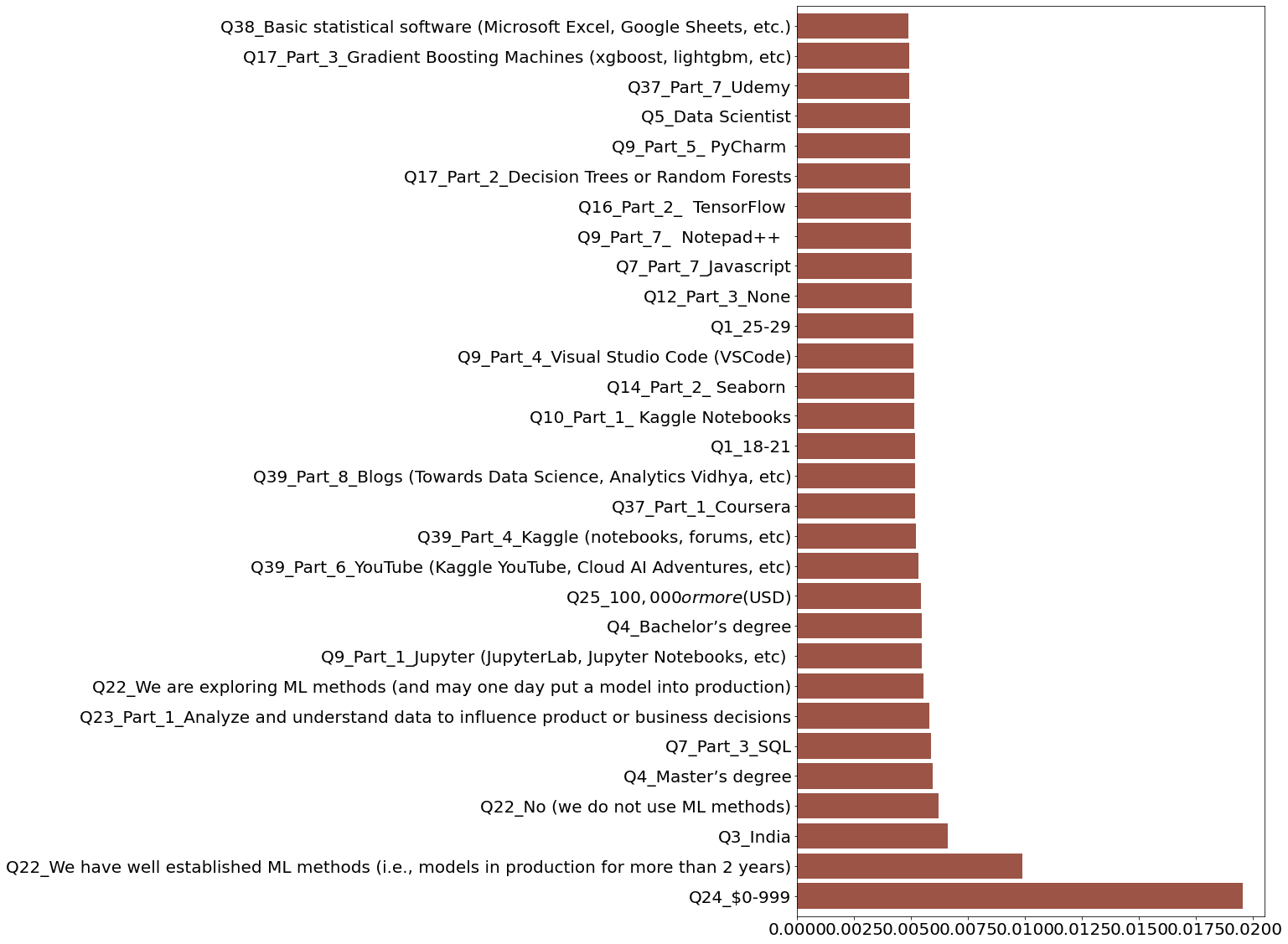
Importance Features:
- Q24_$0-999: Salary
- Q22_We have well established ML methods (i.e., models in production for more than 2 years): Employer incorporate machine learning methods
- Q3_India: Location
- Q22_No (we do not use ML methods): Employer incorporate machine learning methods
- Q4_Master’s degree: Highest level of formal education
- Q7_Part_3_SQL: Programming languages do you use on a regular basis
- Q23_Part_1_Analyze and understand data to influence product or business decisions: Activities that make up an important part of your role at work.
- Q22_We are exploring ML methods (and may one day put a model into production)*: Employer incorporate machine learning methods
- Q9_Part_1_Jupyter (JupyterLab, Jupyter Notebooks, etc)*: Integrated development environments (IDE’s) do you use on a regular basis
- Q4_Bachelor’s degree*: Highest level of formal education
Important Questions:
    important_question = [
        'Q1', 'Q3', 'Q4', 'Q5', 'Q7', 'Q9', 'Q10', 'Q12', 'Q14', 'Q17', 'Q22',
        'Q23', 'Q24', 'Q25', 'Q37', 'Q39'
    ]
Let’s try to use dalex (moDel Agnostic Language for Exploration and eXplanation) to see the break_down plots. The most commonly asked question when trying to understand a model’s prediction for a single observation is: which variables contribute to this result the most?. For that I have used break_down plot from dalex.
exp = dx.Explainer(classifier, X_data, y_data)

bd_large = exp.predict_parts(df[0:1], type='break_down', label="Large Size Company")
bd_mid = exp.predict_parts(df[2:3], type='break_down', label="Mid Size Company")
bd_startup = exp.predict_parts(df[4:5], type='break_down', label="Startup")

k = 20
imps_large = bd_large.result.variable_name.values[1:k + 1].tolist()
imps_mid = bd_mid.result.variable_name.values[1:k + 1].tolist()
imps_startup = bd_startup.result.variable_name.values[1:k + 1].tolist()
results = pd.DataFrame({
    "Large Size Company": [],
    "Mid Size Company": [],
    "Startup": []
})
for ids in zip(imps_large, imps_mid, imps_startup):

    results = results.append(
        pd.DataFrame({
            "Large Size Company": [list(df.columns)[int(ids[0])]],
            "Mid Size Company": [list(df.columns)[int(ids[1])]],
            "Startup": [list(df.columns)[int(ids[2])]]
        }))
Preparation of a new explainer is initiated

  -> data              : numpy.ndarray converted to pandas.DataFrame. Columns are set as string numbers.
  -> data              : 11403 rows 537 cols
  -> target variable   : 11403 values
  -> target variable   : Please note that 'y' is a string array.
  -> target variable   : 'y' should be a numeric or boolean array.
  -> target variable   : Otherwise an Error may occur in calculating residuals or loss.
  -> model_class       : sklearn.ensemble._forest.RandomForestClassifier (default)
  -> label             : Not specified, model's class short name will be used. (default)
  -> predict function  : <function yhat_proba_default at 0x7f3b4f54c3b0> will be used (default)
  -> predict function  : Accepts pandas.DataFrame and numpy.ndarray.
  -> predicted values  : min = 0.0, mean = 0.265, max = 0.91
  -> model type        : classification will be used (default)
  -> residual function : difference between y and yhat (default)
  -> residuals         :  'residual_function' returns an Error when executed:
unsupported operand type(s) for -: 'str' and 'float'
  -> model_info        : package sklearn

A new explainer has been created!
results.reset_index(drop=True)
| Large Size Company | Mid Size Company | Startup | |
|---|---|---|---|
| 0 | Q24_$0-999 | Q24_$0-999 | Q24_$0-999 |
| 1 | Q24_100,000-124,999 | Q25_$10,000-$99,999 | Q4_Doctoral degree |
| 2 | Q29_A_Part_11_Amazon Redshift | Q29_A_Part_11_Amazon Redshift | Q5_Research Scientist |
| 3 | Q37_Part_4_DataCamp | Q37_Part_4_DataCamp | Q24_30,000-39,999 |
| 4 | Q19_Part_3_Contextualized embeddings (ELMo, CoVe) | Q7_Part_10_Bash | Q39_Part_9_Journal Publications (peer-reviewed... |
| 5 | Q9_Part_8_ Sublime Text | Q36_Part_9_I do not share my work publicly | Q36_Part_9_I do not share my work publicly |
| 6 | Q29_A_Part_12_Amazon Athena | Q3_India | Q3_India |
| 7 | Q3_India | Q39_Part_11_None | Q22_We use ML methods for generating insights ... |
| 8 | Q1_30-34 | Q1_30-34 | Q37_Part_11_None |
| 9 | Q17_Part_10_Transformer Networks (BERT, gpt-3,... | Q6_5-10 years | Q1_35-39 |
| 10 | Q31_A_Part_1_Amazon QuickSight | Q27_A_Part_1_ Amazon EC2 | Q17_Part_3_Gradient Boosting Machines (xgboost... |
| 11 | Q14_Part_5_ Shiny | Q31_A_Part_5_Tableau | Q22_We have well established ML methods (i.e.,... |
| 12 | Q6_5-10 years | Q37_Part_10_University Courses (resulting in a... | Q33_A_Part_7_No / None |
| 13 | Q27_A_Part_1_ Amazon EC2 | Q15_3-4 years | Q1_18-21 |
| 14 | Q29_A_Part_2_PostgresSQL | Q33_A_Part_7_No / None | Q7_Part_1_Python |
| 15 | Q31_A_Part_5_Tableau | Q1_18-21 | Q8_Python |
| 16 | Q28_A_Part_1_ Amazon SageMaker | Q12_Part_3_None | Q8_R |
| 17 | Q17_Part_3_Gradient Boosting Machines (xgboost... | Q26_A_Part_1_ Amazon Web Services (AWS) | Q16_Part_13_ Tidymodels |
| 18 | Q18_Part_2_Image segmentation methods (U-Net, ... | Q9_Part_5_ PyCharm | Q25_$100,000 or more ($USD) |
| 19 | Q33_A_Part_7_No / None | Q25_$100,000 or more ($USD) | Q16_Part_1_ Scikit-learn |
Now we got top 20 features which contributed to the prediction pobability. But Still we need to figure out what range of value of these features by company category and how these features related to Company categoies.
Demographic & Opportunity Analysis
Now, We have list of importance features, let’s analyze these features with respect to the company categories. I have divided these features into 5 aspects and these are the following aspects:
- Age and Location Aspect: Which age group prefer working in startups and from where are they from?
- Education and Professional Aspect: How much educated people prefer in working in Startups and Mid/Large Size companies?
- Programming Language Aspect: What programming language/framework they uses on daily basis.
- Work Opportunity Aspect: What are the work opportunities in these companies?
- Salary Aspect: How much they are paying?
Age and Location Aspect
Let’s try to figure out which age group interested in Startup and which age group prefer established company
code
```python def add_rectangular_patch(ax, xy, w, h, color, alpha=0.4, lw=3, fill=True): ax.add_patch( Rectangle(xy, w, h, fill=fill, color=color, lw=lw, alpha=alpha)) def add_annotation(ax, text, xy, xytext, facecolor): ax.annotate( text, xy=xy, xycoords='data', fontsize=16, weight='bold', xytext=xytext, textcoords='axes fraction', arrowprops=dict(facecolor=facecolor, shrink=0.05), horizontalalignment='right', verticalalignment='top', ) def add_annotation_v2(ax, text, xy, fontsize, color, weight='bold', verticalalignment='center', horizontalalignment='center'): ax.annotate(text, xy=xy, fontsize=fontsize, color=color, weight=weight, verticalalignment=verticalalignment, horizontalalignment=horizontalalignment) def hide_axes(this_ax): this_ax.set_frame_on(False) this_ax.set_xticks([]) this_ax.set_yticks([]) return this_ax ``` ```python df = pd.crosstab([data['Q1']], [data['Company_Category']]) df1 = df.apply(lambda r: r / r.sum(), axis=0) df2 = df.apply(lambda r: r / r.sum(), axis=1) df2 = df2.reindex(list(df2.index)[::-1]) heatmap_args = dict(annot_kws={"size": 16}, cmap=cm.get_cmap("Greys", 12), cbar=False, annot=True, fmt="d", lw=2, square=False) f, ax = plt.subplots( nrows=2, ncols=3, figsize=(30, 20), ) # ax [0,0] hide_axes(ax[0, 0]) # ax[0,1] df.apply(lambda r: r.sum(), axis=1).plot.barh(ax=ax[0, 1], fontsize=20, color='#9B5445') total = len(data) for p in ax[0, 1].patches: percentage = '{:.1f}%'.format(100 * p.get_width() / total) x = p.get_x() + p.get_width() + 0.02 y = p.get_y() + p.get_height() / 2 ax[0, 1].annotate(percentage, (x, y)) add_rectangular_patch(ax[0, 1], (0, 0.5), 2550, 4, 'darkgreen', alpha=0.4, lw=3) add_annotation(ax[0, 1], '67%', (2400, 5), (0.8, 0.65), 'darkgreen') add_rectangular_patch(ax[0, 1], (0, 1.5), 2550, 2, 'darkred', alpha=0.4, lw=3) add_annotation(ax[0, 1], '40%', (1000, 3), (0.6, 0.65), 'darkred') # ax[0,2] hide_axes(ax[0, 2]) # ax[1,0] df1.transpose()[list(df1.transpose().columns)[::-1]].plot.bar(ax=ax[1, 0], stacked=True, fontsize=20, colormap=cm.get_cmap("tab20", 20)) ax[1,0].legend(fontsize=20, handlelength=1,labelspacing =0.2, loc='upper right', bbox_to_anchor=(0.5, 0.6)) add_rectangular_patch(ax[1, 0], (-0.5, 0.45), 2, 0.4, 'darkgreen', alpha=0.2, lw=5, fill=True) add_rectangular_patch(ax[1, 0], (1.5, 0.73), 1, 0.27, 'darkred', alpha=0.2, lw=5, fill=True) # ax[1,1] midpoint = (df.values.max() - df.values.min()) / 2 hm = sns.heatmap(df, ax=ax[1, 1], center=midpoint, **heatmap_args) hm.set_xticklabels(hm.get_xmajorticklabels(), fontsize=20, rotation=90) hm.set_yticklabels(hm.get_ymajorticklabels(), fontsize=20, rotation=0) # ax[1,2] df2.plot.barh(ax=ax[1, 2], fontsize=20, stacked=True) ax[1,2].legend(fontsize=20, handlelength=1,labelspacing =0.2, loc=6) add_rectangular_patch(ax[1, 2], (0, 8.5), 1, 1.9, 'darkgreen', alpha=0.2, lw=5, fill=True) add_annotation_v2(ax[1, 2], 'Learning-First', (0.5, 9.5), fontsize=40, color='white', weight='bold', verticalalignment='center', horizontalalignment='center') add_rectangular_patch(ax[1, 2], (0, 2.5), 1, 5.9, 'darkred', alpha=0.2, lw=5, fill=True) add_annotation_v2(ax[1, 2], 'Stability-First', (0.5, 6.5), fontsize=40, color='white', weight='bold', verticalalignment='center', horizontalalignment='center') add_rectangular_patch(ax[1, 2], (0, 0), 1, 2.5, 'darkgreen', alpha=0.2, lw=5, fill=True) add_annotation_v2(ax[1, 2], "Let's-Do-Startup", (0.5, 1.0), fontsize=40, color='white', weight='bold', verticalalignment='center', horizontalalignment='center') title = f.suptitle('Learning First or Stability First', fontsize=30) ```
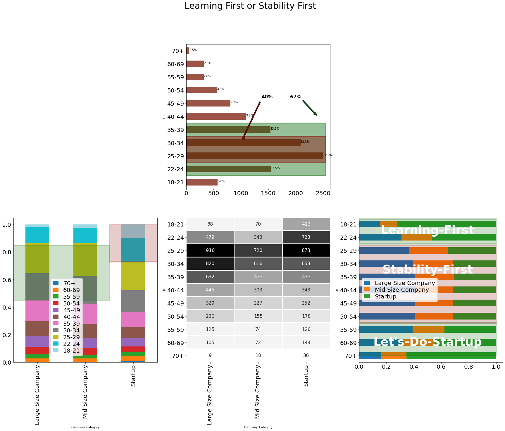
🚀Highlights:
- 67% of respondents age are b/w 22-40 and 40% are in 25-34
- 5 out of 10 in Large and Mid size company are of age b/w 25-34, where as 3 out of 10 in Startup has employee of age b/w 18-24
- More than ~50% of respondents having age b/w 18-24 are working in Startup, whereas more than ~60% having age b/w 25-54 are working in either in Mid or Large size company. It feels like in the starting of career they want to learn lots of different things and after 25 they go for stability in life for work-life balance.
- There is an interesting pattern after 55, Looks like people again want to learn and discover new thing and want to get rid of corporate culture and go for the startup.
code
```python df = pd.crosstab([data['Q3']], [data['Company_Category']]) df = df.reindex(df.sum(axis=1).sort_values().index) ax = df.plot.barh( stacked=True, figsize=(15, 15), width=0.85, ) ax.spines['right'].set_visible(False) ax.spines['top'].set_visible(False) ax.spines['left'].set_visible(False) ax.spines['bottom'].set_visible(False) title = ax.title.set_text('Does India or USA has more respondents') ```
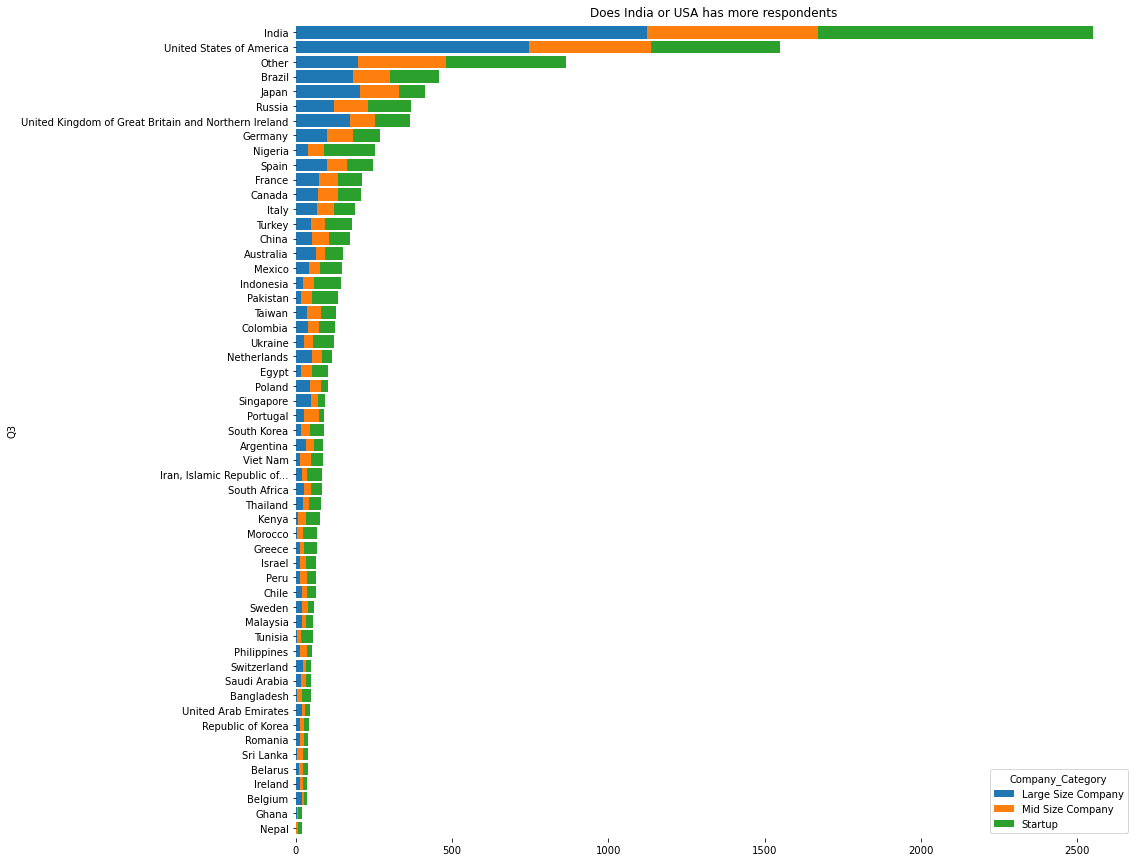
🚀Highlights:
- ~35 of respondents are from India or USA
- Distrubtion of Company category looks balanced b/w Country wise respondents
⚡Inference:
In the starting (18-24) of carrier people go for Startups to learn and experiment new things, in middle(25-34) they go to establish company for maintaining work life balance because that time they likely to have families n all and in last(50+) they again go for Startups, in this time they likely to have some idea for entrepreneur and they want to implement that.
Education and Professional Aspect
Now Let’s try to figure out how formal education are distrubuted over company category. Do they actualy perfer Master or PhDs or they also consider bachelors.
code
```python df = pd.crosstab([data['Q4']], [data['Company_Category']]) df1 = df.apply(lambda r: r/r.sum(), axis=0) df2 = df.apply(lambda r: r/r.sum(), axis=1) f, ax = plt.subplots( nrows=2, ncols=3, figsize=(30, 20), ) hide_axes(ax[0, 0]) df.apply(lambda r: r.sum(), axis=1).plot.barh(ax=ax[0, 1], fontsize=20, color='#9B5445') total = len(data) for p in ax[0, 1].patches: percentage = '{:.1f}%'.format(100 * p.get_width()/total) x = p.get_x() + p.get_width() + 0.02 y = p.get_y() + p.get_height()/2 ax[0, 1].annotate(percentage, (x, y)) hide_axes(ax[0, 2]) df.plot.bar(ax=ax[1, 0], fontsize=20) ax[1,0].legend(fontsize=20, handlelength=1,labelspacing =0.2) df1.transpose().plot.bar(ax=ax[1, 1], fontsize=20, stacked=True, colormap=cm.get_cmap("tab20", 20)) ax[1,1].legend(fontsize=13, handlelength=1, labelspacing =0.2, loc=10) df2.plot.bar(ax=ax[1, 2], fontsize=20, stacked=True) ax[1,2].legend(fontsize=20, handlelength=1,labelspacing =0.2) add_rectangular_patch(ax[1, 2], (-0.5, 0.45), 2, 0.6, 'darkgreen', alpha=0.2, lw=5, fill=True) title = f.suptitle('Master/PhD or Bachelor is enough?', fontsize=30) ```
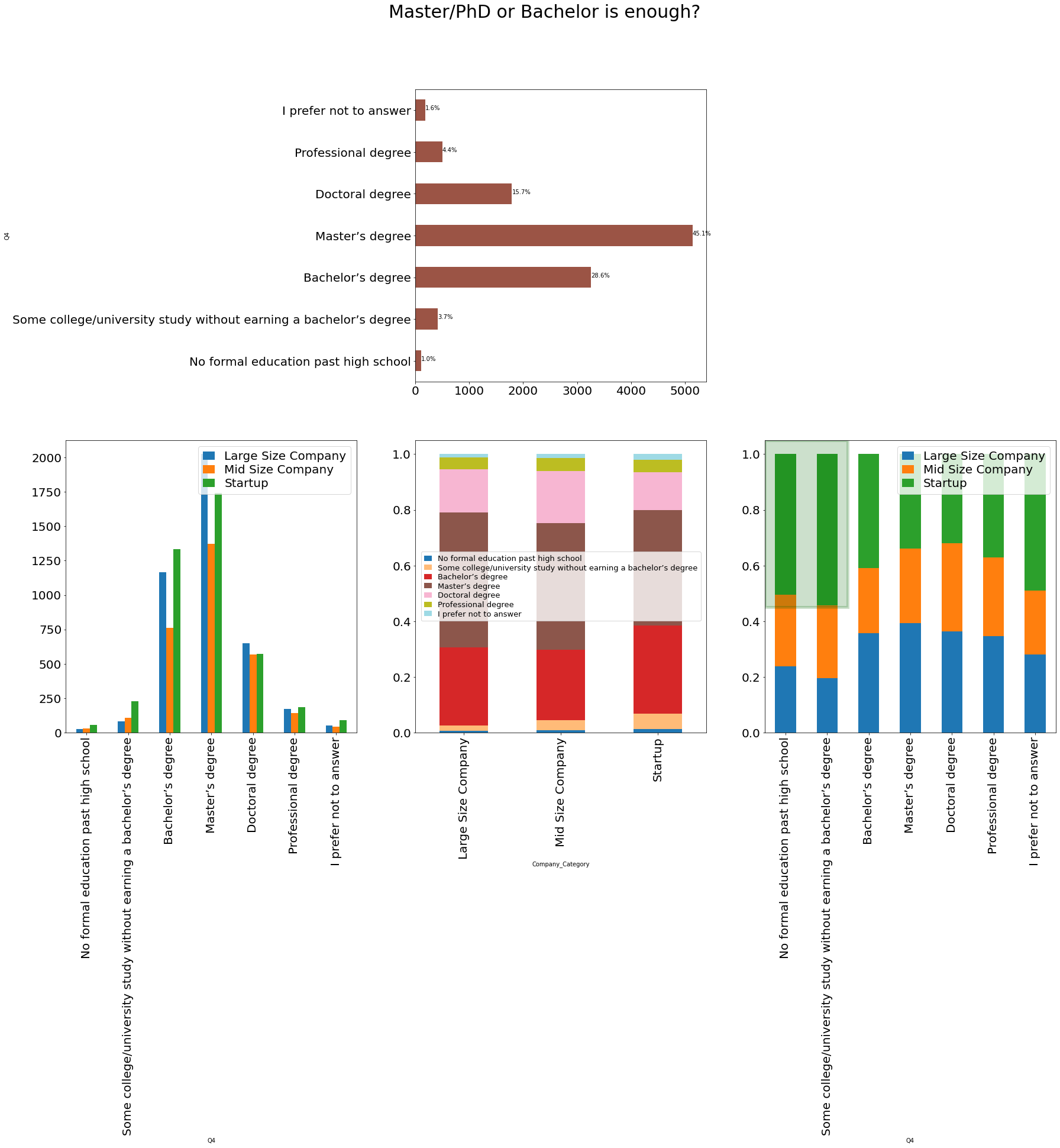
🚀Highlights:
- ~45% respondents have completed Master’s Dregree.
- Startups has more bachelors and less Master’s & PhD’s compare to Large and Mid Size company.
- The respondents who have’nt completed either high school or bachelors are mostly work for Startups.
code
```python def get_count_dfs(data, col1, col2): df = pd.crosstab([data[col1]], [data[col2]]) df1 = df.apply(lambda r: r / r.sum(), axis=0) df2 = df.apply(lambda r: r / r.sum(), axis=1) return df, df1, df2 def reindex_df(df, reverse=False): if reverse: df = df.reindex(list(df.sum(axis=1).sort_values().index)[::-1]) return df df = df.reindex(df.sum(axis=1).sort_values().index) return df main_col = "Company_Category" by_col = "Q5" by_col2 = "Q4" index_cols = ['Software Engineer', 'DBA/Database Engineer', 'Data Engineer', 'Machine Learning Engineer', 'Statistician', 'Data Analyst', 'Data Scientist', 'Research Scientist', 'Business Analyst', 'Product/Project Manager', 'Other'] df, df1, df2 = get_count_dfs(data, by_col, main_col) df = df.reindex(index_cols) df1 = df1.reindex(index_cols) df2 = df2.reindex(index_cols) df3 = pd.crosstab([data[by_col]], [data[by_col2]]) df3 = df3.reindex(index_cols) heatmap_args = dict(annot=True, fmt="d", square=False, cmap=cm.get_cmap("Greys", 12), center=90, vmin=0, vmax=500, lw=4, cbar=False) f, ax = plt.subplots(nrows=2, ncols=3, figsize=(30, 20), gridspec_kw={ 'height_ratios': [4, 6], 'wspace': 0.6, 'hspace': 0.6 }) # ax[0,0] df = df.reindex(index_cols[::-1]) df.apply(lambda r: r.sum(), axis=1).plot.barh(ax=ax[0, 0], fontsize=20, color='#9B5445') total = len(data) for p in ax[0, 0].patches: percentage = '{:.1f}%'.format(100 * p.get_width() / total) x = p.get_x() + p.get_width() + 0.02 y = p.get_y() + p.get_height() / 2 ax[0, 0].annotate(percentage, (x, y)) # ax[0,1] hm = sns.heatmap(df3, ax=ax[0, 1], annot_kws={"size": 16}, **heatmap_args) hm.set_xticklabels(hm.get_xmajorticklabels(), fontsize=20) hm.set_yticklabels(hm.get_ymajorticklabels(), fontsize=20) add_rectangular_patch(ax[0, 1], (0, 5), 2, 2, 'yellow', alpha=0.1, lw=5, fill=True) # ax[0,2] df3.apply(lambda r: r.sum(), axis=0).plot.bar(ax=ax[0, 2], fontsize=20, color='#9B5445') total = len(data) for p in ax[0, 2].patches: percentage = '{:.1f}%'.format(100 * p.get_height() / total) x = p.get_x() + p.get_width() - 0.5 y = p.get_y() + p.get_height() + 100 ax[0, 2].annotate(percentage, (x, y)) # ax[1,0] df = df.reindex(index_cols) df.plot.bar(ax=ax[1, 0], fontsize=20, width=0.65) ax[1,0].legend(fontsize=20, handlelength=1,labelspacing =0.2, loc=1) add_rectangular_patch(ax[1, 0], (2.5, 0), 1, 600, 'darkgreen', alpha=0.2, lw=5, fill=True) # ax[1,1] df1.transpose().plot.bar(ax=ax[1, 1], stacked=True,colormap=cm.get_cmap("tab20", 12), fontsize=20, width=0.65) ax[1,1].legend(fontsize=13, handlelength=1, labelspacing =0.2, loc=1) # ax[1,2] df2.plot.bar(ax=ax[1, 2], fontsize=20, stacked=True, width=0.65) ax[1,2].legend(fontsize=20, handlelength=1,labelspacing =0.2, loc=1) title = f.suptitle('Data Scientist or Software Engineer or ML Engineer?', fontsize=30) ```
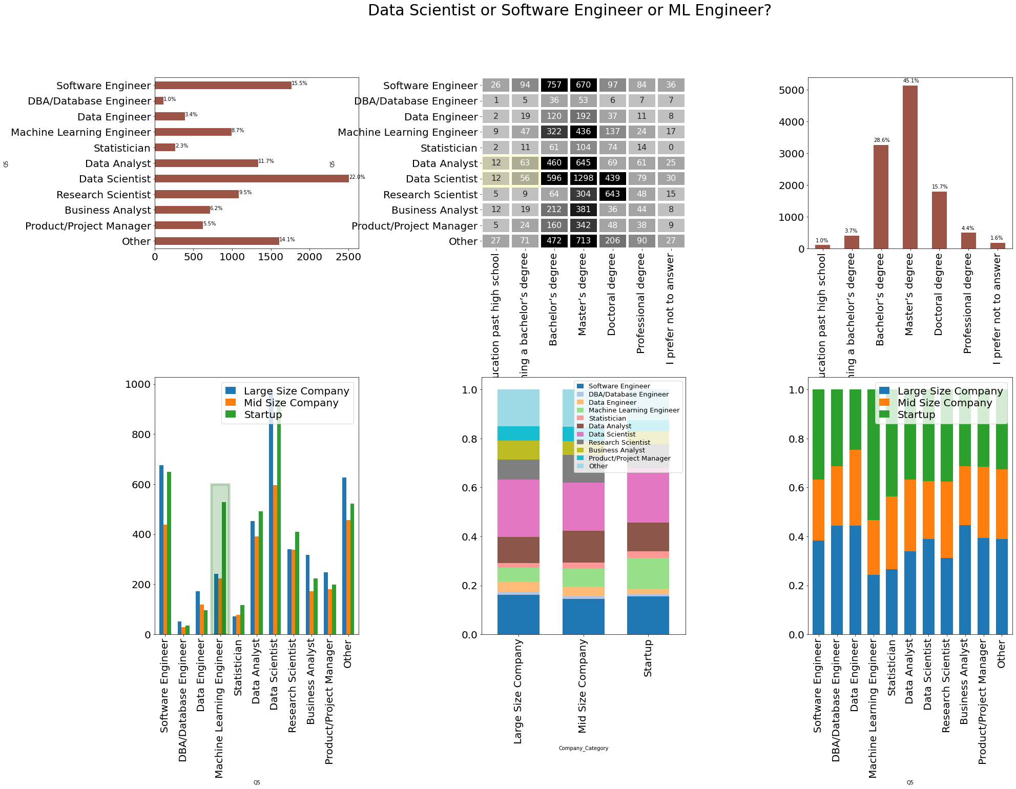
🚀Highlights:
- ~22% data scientist and ~16% software developer respondents.
- ~1.5% of respondents has not compeleted thier high school or bachelor’s and working as Data scientist or Analyst.
- Startups has more number of Machine Learning Engineers compare to Mid or Large Size company.
- ~40% of Research Scientist are from Startups.
- More Business Analyst Profiles are in Large Size Company.
Programming Language Aspect
code
```python df = pd.crosstab([data['Q6']], [data['Company_Category']]) df1 = df.apply(lambda r: r/r.sum(), axis=0) df2 = df.apply(lambda r: r/r.sum(), axis=1) df = df.reindex(list(df.index)[::-1] ) df_ = pd.crosstab([data['Q15']], [data['Company_Category']]) df1_ = df_.apply(lambda r: r/r.sum(), axis=0) df2_ = df_.apply(lambda r: r/r.sum(), axis=1) df_ = df_.reindex(list(df_.index)[::-1] ) heatmap_args = dict(annot_kws={"size": 16}, cmap=cm.get_cmap("Greys", 12), cbar=False, annot=True, fmt="d", lw=2, square=False) f, ax = plt.subplots(nrows=2, ncols=3, figsize=(30, 20), gridspec_kw={ 'height_ratios': [5, 5], 'wspace': 0.6, 'hspace': 0.6 }) # ax[0,0] df1.transpose().plot.bar(ax=ax[0, 0], fontsize=20, stacked=True, width=0.65, colormap=cm.get_cmap("tab20", 20)) # ax[0,1] midpoint = (df.values.max() - df.values.min()) / 2 hm = sns.heatmap(df, ax=ax[0, 1], center=midpoint, **heatmap_args) hm.set_xticklabels(hm.get_xmajorticklabels(), fontsize=20, rotation=90) hm.set_yticklabels(hm.get_ymajorticklabels(), fontsize=20, rotation=0) # ax[0,2] df2.plot.barh(ax=ax[0, 2], fontsize=20, width=0.65, stacked=True) # ax[1,0] df1_.transpose().plot.bar(ax=ax[1, 0], fontsize=20, stacked=True, width=0.65, colormap=cm.get_cmap("tab20", 20)) # ax[1,1] midpoint_ = (df_.values.max() - df_.values.min()) / 2 hm_ = sns.heatmap(df_, ax=ax[1, 1], center=midpoint_, **heatmap_args) hm_.set_xticklabels(hm_.get_xmajorticklabels(), fontsize=20, rotation=90) hm_.set_yticklabels(hm_.get_ymajorticklabels(), fontsize=20, rotation=0) # ax[1,2] df2_.plot.barh(ax=ax[1, 2], fontsize=20, width=0.65, stacked=True) title = f.suptitle('Coding experience or ML experience?', fontsize=30) ```
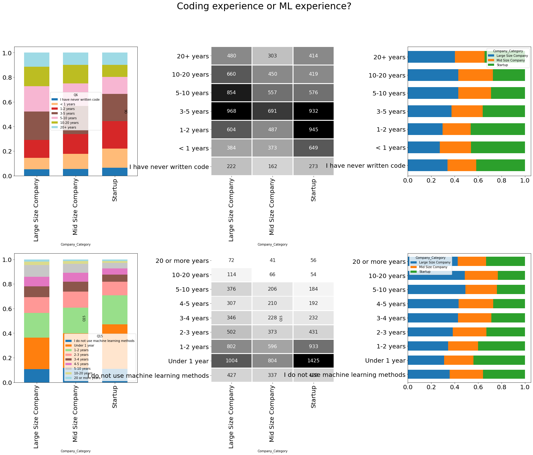
🚀Highlights:
- ~40% of employee of Large size company are of 3-10 years coding experience.
- ~60% of employee of Startup are under 5 years of coding experience.
- ~50% of respondents having 0-2 years of coding experience works in Startup.
- ~30% of employee of Large size company are of 0-1 year of Machine Learning Experience.
- ~40% of employee of Startup are of 0-1 year of Machine Learning Experience.
code
```python def get_df_for_multi_part_question(data, main_col, by_col): cols = get_columns(by_col) + [main_col] df = data[cols] df = (df.set_index(["Company_Category"]).stack().reset_index(name='Value')) del df['level_1'] df.columns = [main_col, by_col] df = pd.crosstab([df[by_col]], [df['Company_Category']]) df = df.reindex(df.sum(axis=1).sort_values().index) return df q7_df = get_df_for_multi_part_question(data, "Company_Category", "Q7") q9_df = get_df_for_multi_part_question(data, "Company_Category", "Q9") q14_df = get_df_for_multi_part_question(data, "Company_Category", "Q14") q16_df = get_df_for_multi_part_question(data, "Company_Category", "Q16") f, ax = plt.subplots(nrows=2, ncols=2, figsize=(20, 20), gridspec_kw={ 'height_ratios': [5, 5], 'wspace': 0.4, 'hspace': 0.1 }) # ax[0,0] (q9_df/data['Company_Category'].value_counts()).plot.barh(ax=ax[0, 0], fontsize=20, width=0.65) # ax[0,1] (q7_df/data['Company_Category'].value_counts()).plot.barh(ax=ax[0, 1], fontsize=20, width=0.65) # ax[1,0] (q14_df/data['Company_Category'].value_counts()).plot.barh(ax=ax[1, 0], fontsize=20, width=0.65) # ax[1,1] (q16_df/data['Company_Category'].value_counts()).plot.barh(ax=ax[1, 1], fontsize=20, width=0.65) title = f.suptitle('R vs Python & SKLearn or Tensorflow/Keras/Pytorch', fontsize=30) ```
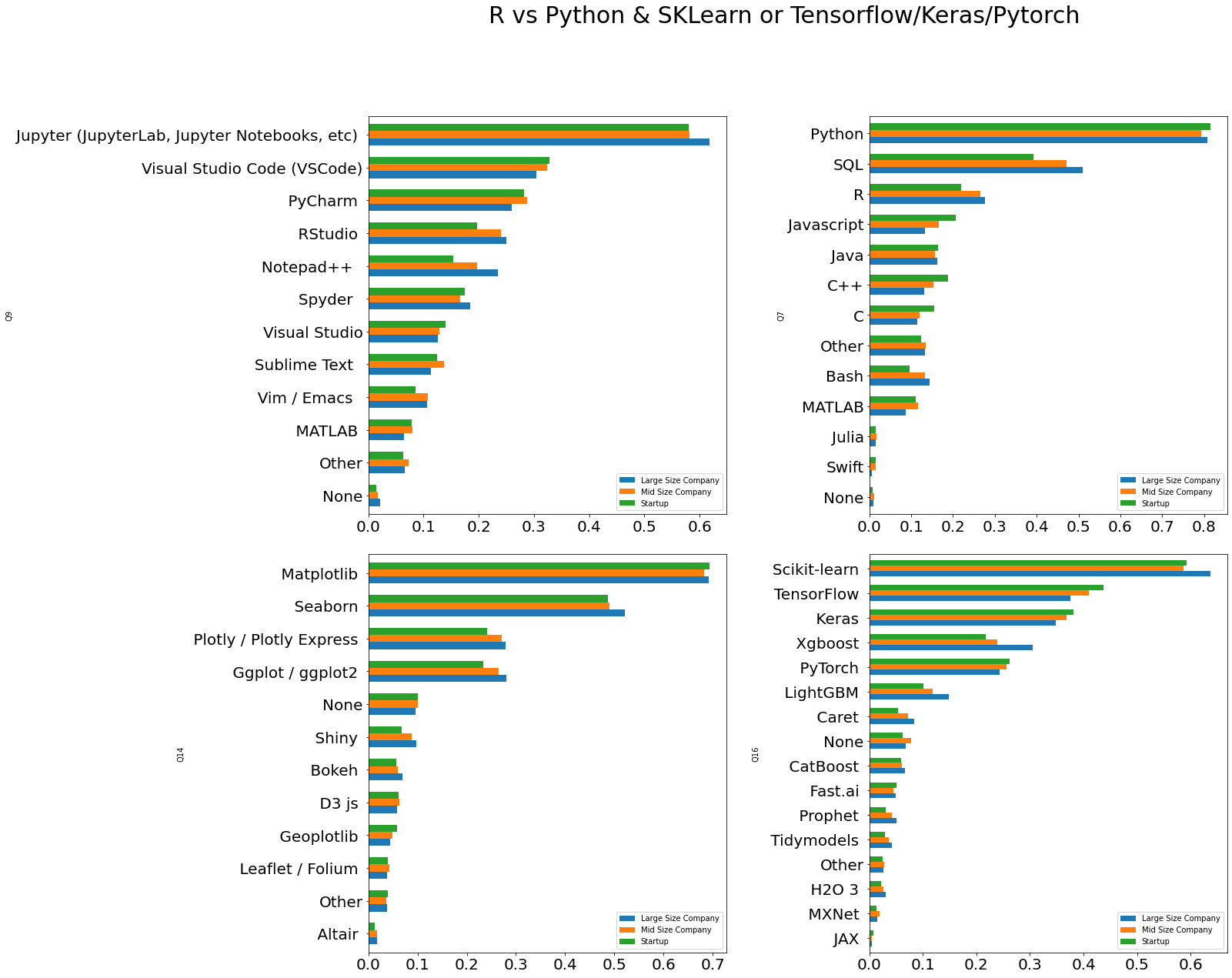
🚀Highlights:
- More large size company uses Jupyter Notebook comare to Startup & Mid size company.
- Significant number of large size company uses Notepad++.
- SQL & R are more used in Large Size Company.
- Scikit-Learn, Xgboost, LightGBM, Caret, Catboost are more used in Large Size Company.
- Tensorflow, Keras, Pytorch are more used in Startups.
Work Opportunity Aspect
code
```python df = pd.crosstab([data['Q21']], [data['Company_Category']]) df1 = df.apply(lambda r: r/r.sum(), axis=0) df2 = df.apply(lambda r: r/r.sum(), axis=1) def hide_axes(this_ax): this_ax.set_frame_on(False) this_ax.set_xticks([]) this_ax.set_yticks([]) return this_ax f, ax = plt.subplots( nrows=2, ncols=3, figsize=(30, 20), ) hide_axes(ax[0, 0]) df.apply(lambda r: r.sum(), axis=1).plot.barh(ax=ax[0, 1], fontsize=20, color='#9B5445') total = len(data) for p in ax[0, 1].patches: percentage = '{:.1f}%'.format(100 * p.get_width()/total) x = p.get_x() + p.get_width() + 0.02 y = p.get_y() + p.get_height()/2 ax[0, 1].annotate(percentage, (x, y)) hide_axes(ax[0, 2]) df.plot.bar(ax=ax[1, 0], fontsize=20) df1.transpose().plot.bar(ax=ax[1, 1], fontsize=20, stacked=True, colormap=cm.get_cmap("tab20", 20)) df2.plot.bar(ax=ax[1, 2], fontsize=20, stacked=True) title = f.suptitle('len(ML Workforce)?', fontsize=30) ```
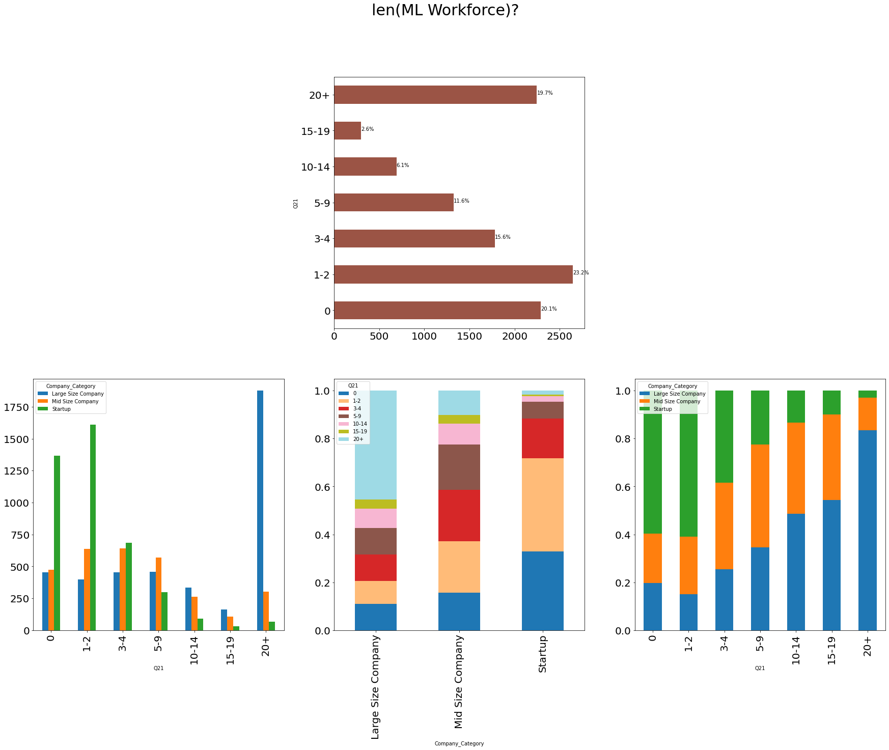
🚀Highlights:
- Mostly startup has 0-2 people are responsible for the data science workloads.
- 20+ People included in Large Size Company for the data science workloads
- >50% of Mid size company has 0-4 People are responsible for the data science workloads.
code
```python df = pd.crosstab([data['Q22']], [data['Company_Category']]) df1 = df.apply(lambda r: r / r.sum(), axis=0) df2 = df.apply(lambda r: r / r.sum(), axis=1) def hide_axes(this_ax): this_ax.set_frame_on(False) this_ax.set_xticks([]) this_ax.set_yticks([]) return this_ax f, ax = plt.subplots(nrows=2, ncols=3, figsize=(30, 20), gridspec_kw={ 'height_ratios': [5, 5], 'wspace': 0.2, 'hspace': 0.1 }) hide_axes(ax[0, 0]) df = reindex_df(df) df.apply(lambda r: r.sum(), axis=1).plot.barh(ax=ax[0, 1], fontsize=20, color='#9B5445') total = len(data) for p in ax[0, 1].patches: percentage = '{:.1f}%'.format(100 * p.get_width() / total) x = p.get_x() + p.get_width() + 0.02 y = p.get_y() + p.get_height() / 2 ax[0, 1].annotate(percentage, (x, y)) hide_axes(ax[0, 2]) df = reindex_df(df, True) df1 = reindex_df(df1, True) df2 = reindex_df(df2, True) df.plot.bar(ax=ax[1, 0], fontsize=20) df1.transpose().plot.bar(ax=ax[1, 1], fontsize=20, colormap=cm.get_cmap("tab20", 20), stacked=True) df2.plot.bar(ax=ax[1, 2], fontsize=20, stacked=True) title = f.suptitle('Do they incorporated Machine Learning?', fontsize=30) ```
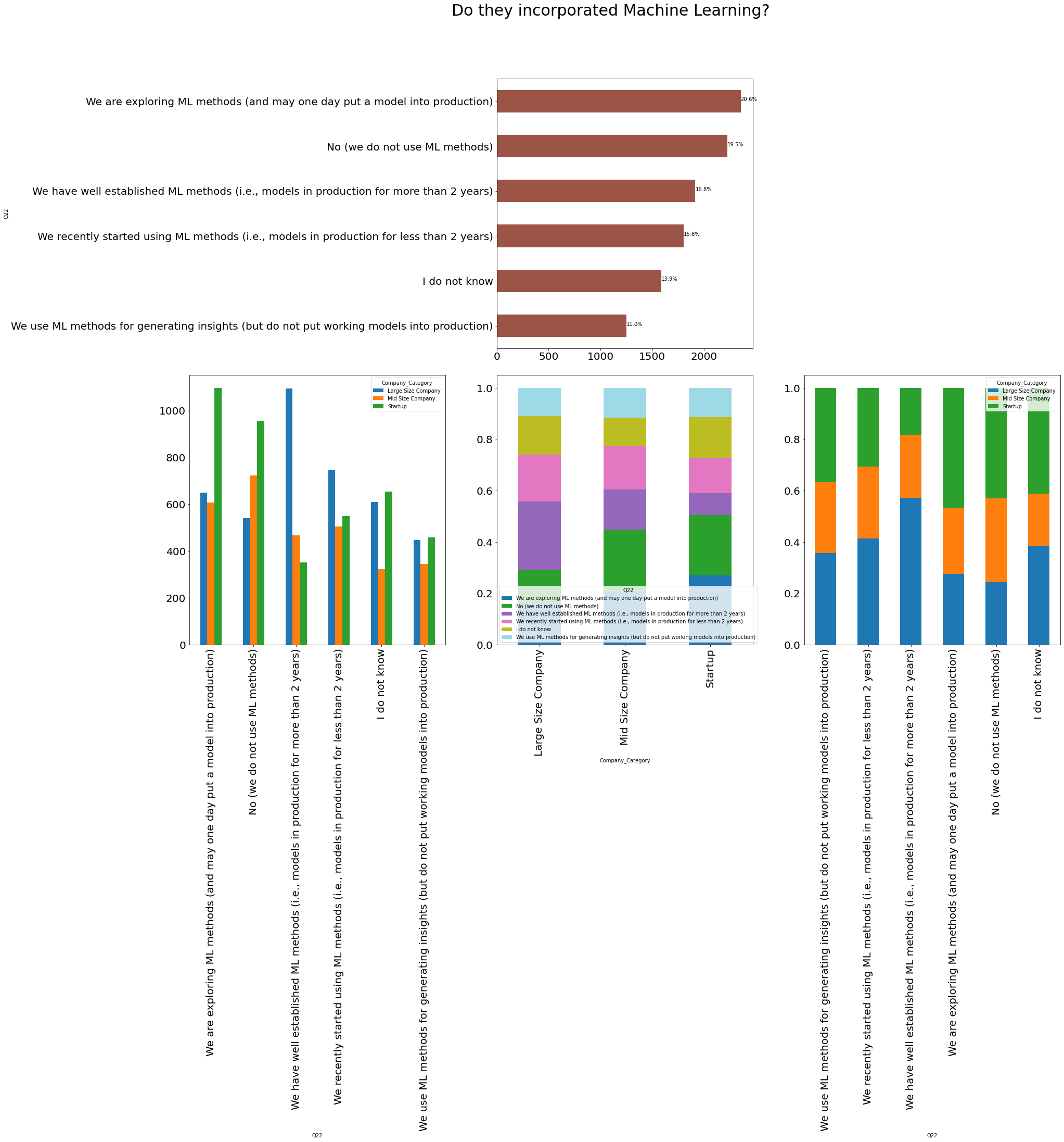
🚀Highlights:
- ~30% Startups are exploring ML methods and may one day put a model into production.
- ~25% Large Size company has have well established ML methods and models in production for more than 2 years.
code
```python main_col = "Company_Category" by_col = "Q23" cols = get_columns(by_col) + [main_col] df = data[cols] df = (df.set_index(["Company_Category"]).stack().reset_index(name='Value')) del df['level_1'] df.columns = [main_col, by_col] df = pd.crosstab([df[by_col]], [df['Company_Category']]) df1 = df.apply(lambda r: r / r.sum(), axis=0) df2 = df.apply(lambda r: r / r.sum(), axis=1) def hide_axes(this_ax): this_ax.set_frame_on(False) this_ax.set_xticks([]) this_ax.set_yticks([]) return this_ax f, ax = plt.subplots(nrows=2, ncols=3, figsize=(30, 20), gridspec_kw={ 'height_ratios': [5, 5], 'wspace': 0.1, 'hspace': 0.2 }) hide_axes(ax[0, 0]) df = reindex_df(df) df.apply(lambda r: r.sum(), axis=1).plot.barh(ax=ax[0, 1], fontsize=20, color='#9B5445') total = len(data) for p in ax[0, 1].patches: percentage = '{:.1f}%'.format(100 * p.get_width() / total) x = p.get_x() + p.get_width() + 0.02 y = p.get_y() + p.get_height() / 2 ax[0, 1].annotate(percentage, (x, y)) hide_axes(ax[0, 2]) df = reindex_df(df, True) df1 = reindex_df(df1, True) df2 = reindex_df(df2, True) df.plot.bar(ax=ax[1, 0], fontsize=20) (df/data['Company_Category'].value_counts()).plot.bar(ax=ax[1, 1], fontsize=20) df2.plot.bar(ax=ax[1, 2], fontsize=20, stacked=True) title = f.suptitle('What they doing?', fontsize=30) ```
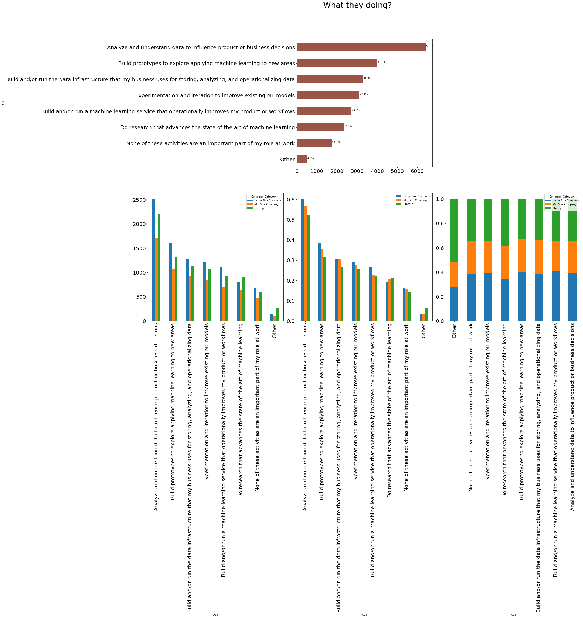
🚀Highlights:
- 56% of Companies are Analyzing and understanding data to influence product or business decisions.
- 40% of Large size company and 30% of Startup are building prototypes to explore applying machine learning to new areas.
Salary Aspect
Let’s us see how salary varies with the companay size.
Starting with job role. To calculate salary part, I used reponse of Q24 and took upper bound as thier salary for simlicity and NaN repaced with the mean value. Now with the use of groupy function of pandas, I able to calculate salary by job role and company category.
code
```python salary_in_order = [ "$0-999", "1,000-1,999", "2,000-2,999", "3,000-3,999", "4,000-4,999", "5,000-7,499", "7,500-9,999", "10,000-14,999", "15,000-19,999", "20,000-24,999", "25,000-29,999", "30,000-39,999", "40,000-49,999", "50,000-59,999", "60,000-69,999", "70,000-79,999", "80,000-89,999", "90,000-99,999", "100,000-124,999", "125,000-149,999", "150,000-199,999", "200,000-249,999", "300,000-500,000", "> $500,000", "nan" ] ## Put NaN with mean salary_in_value = [ 999, 1999, 2999, 3999, 4999, 7499, 9999, 14999, 19999, 24999, 29999, 39999, 49999, 59999, 69999, 79999, 89999, 99999, 124999, 149999, 199999, 249999, 500000, 1000000, 46910 ] salary_lookup = dict(zip(salary_in_order, salary_in_value)) data['Q24_new'] = data['Q24'].astype(str) data['Q24_new'] = data['Q24_new'].apply(lambda x: salary_lookup[x]) ``` ```python def add_annotation(ax, text, xy, xytext, facecolor): ax.annotate( text, xy=xy, xycoords='data', fontsize=16, weight=None, xytext=xytext, textcoords='axes fraction', arrowprops=dict(facecolor=facecolor, shrink=0.05), horizontalalignment='right', verticalalignment='top', ) ``` ```python df = data[['Company_Category','Q5', 'Q24_new']].groupby(['Company_Category','Q5']).describe() df = df['Q24_new'] (df.style .background_gradient(subset=['mean'])) ```
| count | mean | std | min | 25% | 50% | 75% | max | ||
|---|---|---|---|---|---|---|---|---|---|
| Company_Category | Q5 | ||||||||
| Large Size Company | Business Analyst | 317.000 | 48365.735 | 54009.599 | 999.000 | 9999.000 | 39999.000 | 69999.000 | 500000.000 |
| DBA/Database Engineer | 51.000 | 66438.451 | 140567.291 | 999.000 | 14999.000 | 39999.000 | 69999.000 | 1000000.000 | |
| Data Analyst | 452.000 | 44258.460 | 50615.318 | 999.000 | 7499.000 | 24999.000 | 59999.000 | 500000.000 | |
| Data Engineer | 173.000 | 63913.451 | 89405.007 | 999.000 | 14999.000 | 46910.000 | 79999.000 | 1000000.000 | |
| Data Scientist | 978.000 | 79224.119 | 95688.852 | 999.000 | 19999.000 | 54999.000 | 124999.000 | 1000000.000 | |
| Machine Learning Engineer | 241.000 | 72179.232 | 115729.684 | 999.000 | 7499.000 | 39999.000 | 89999.000 | 1000000.000 | |
| Other | 627.000 | 61932.820 | 91976.007 | 999.000 | 7499.000 | 39999.000 | 79999.000 | 1000000.000 | |
| Product/Project Manager | 247.000 | 80123.745 | 74590.717 | 999.000 | 29999.000 | 69999.000 | 124999.000 | 500000.000 | |
| Research Scientist | 340.000 | 79595.779 | 146005.220 | 999.000 | 14999.000 | 46910.000 | 82499.000 | 1000000.000 | |
| Software Engineer | 675.000 | 56162.613 | 111186.941 | 999.000 | 7499.000 | 24999.000 | 59999.000 | 1000000.000 | |
| Statistician | 71.000 | 71181.634 | 81723.700 | 999.000 | 12499.000 | 49999.000 | 99999.000 | 500000.000 | |
| Mid Size Company | Business Analyst | 172.000 | 45950.942 | 85187.530 | 999.000 | 7499.000 | 24999.000 | 59999.000 | 1000000.000 |
| DBA/Database Engineer | 28.000 | 76641.893 | 187652.780 | 999.000 | 3749.000 | 24999.000 | 67499.000 | 1000000.000 | |
| Data Analyst | 391.000 | 33407.350 | 38283.207 | 999.000 | 2999.000 | 14999.000 | 49999.000 | 249999.000 | |
| Data Engineer | 120.000 | 52999.467 | 65660.127 | 999.000 | 7499.000 | 29999.000 | 79999.000 | 500000.000 | |
| Data Scientist | 595.000 | 64784.402 | 92530.380 | 999.000 | 14999.000 | 39999.000 | 89999.000 | 1000000.000 | |
| Machine Learning Engineer | 223.000 | 50853.206 | 65934.683 | 999.000 | 3999.000 | 29999.000 | 59999.000 | 500000.000 | |
| Other | 457.000 | 51604.140 | 94100.363 | 999.000 | 3999.000 | 19999.000 | 59999.000 | 1000000.000 | |
| Product/Project Manager | 181.000 | 67920.000 | 95610.307 | 999.000 | 9999.000 | 46910.000 | 89999.000 | 1000000.000 | |
| Research Scientist | 338.000 | 41034.728 | 50834.413 | 999.000 | 2999.000 | 19999.000 | 59999.000 | 249999.000 | |
| Software Engineer | 439.000 | 45799.708 | 91669.747 | 999.000 | 3999.000 | 24999.000 | 59999.000 | 1000000.000 | |
| Statistician | 79.000 | 38173.962 | 45869.644 | 999.000 | 3999.000 | 14999.000 | 59999.000 | 199999.000 | |
| Startup | Business Analyst | 223.000 | 40505.682 | 89929.708 | 999.000 | 999.000 | 9999.000 | 46910.000 | 1000000.000 |
| DBA/Database Engineer | 36.000 | 32688.500 | 41397.226 | 999.000 | 1999.000 | 14999.000 | 49999.000 | 149999.000 | |
| Data Analyst | 492.000 | 22609.541 | 55265.584 | 999.000 | 999.000 | 2999.000 | 29999.000 | 1000000.000 | |
| Data Engineer | 96.000 | 44424.812 | 72132.595 | 999.000 | 1749.000 | 14999.000 | 59999.000 | 500000.000 | |
| Data Scientist | 937.000 | 41081.572 | 97318.933 | 999.000 | 999.000 | 7499.000 | 46910.000 | 1000000.000 | |
| Machine Learning Engineer | 528.000 | 24833.379 | 47422.643 | 999.000 | 999.000 | 2999.000 | 39999.000 | 500000.000 | |
| Other | 522.000 | 39493.249 | 86954.872 | 999.000 | 999.000 | 14999.000 | 46910.000 | 1000000.000 | |
| Product/Project Manager | 198.000 | 51205.283 | 89628.317 | 999.000 | 2999.000 | 24999.000 | 59999.000 | 1000000.000 | |
| Research Scientist | 410.000 | 42202.039 | 108386.977 | 999.000 | 999.000 | 9999.000 | 46910.000 | 1000000.000 | |
| Software Engineer | 650.000 | 30492.631 | 43956.411 | 999.000 | 999.000 | 9999.000 | 46910.000 | 500000.000 | |
| Statistician | 116.000 | 23055.991 | 59313.111 | 999.000 | 999.000 | 999.000 | 26249.000 | 500000.000 |
🚀Highlights:
-
Average Salary in Large Size Company are Research Scientist(77741) > Data Scientist(77737) > Machine Learning Engineer(73560) > Statistician(71181) > Data Engineer(63187) > Data Analyst (44106)
-
Average Salary in Mid Size Company are Data Scientist(64432) > Data Engineer(53419) > Machine Learning Engineer(51064) > Research Scientist(40375) > Statistician(38650) > Data Analyst(33369)
-
Average Salary in Startup are Data Scientist(41170) > Research Scientist(41550) > Data Engineer(39629) > Machine Learning Engineer(24921) > Statistician(23247) > Data Analyst(22645)
-
Product/Project Manager get more money
code
```python %matplotlib inline %config InlineBackend.figure_format='retina' index_cols = ['Software Engineer', 'DBA/Database Engineer', 'Data Engineer', 'Machine Learning Engineer', 'Statistician', 'Data Analyst', 'Data Scientist', 'Research Scientist', 'Business Analyst', 'Product/Project Manager', 'Other'] data['Q5'] = pd.Categorical(data['Q5'], categories=index_cols, ordered=True) df = pd.crosstab([data['Q24'], data['Company_Category'], data['Q5']], []).reset_index() df = df.rename(columns={'__dummy__': 'size'}) df1 = pd.crosstab([data['Company_Category'], data['Q5']], []).reset_index() df1 = df1.rename(columns={'__dummy__': 'total_size'}) df = df.merge(df1, how='inner', on=['Company_Category', 'Q5']) df['percentage'] = df['size']/df['total_size'] palette = sns.color_palette("tab20", len(data['Q5'].unique())) lp = sns.relplot( data=df, x="Q24", y="percentage", hue="Q5", col="Company_Category", kind="scatter", height=5, aspect=.75, palette=palette, facet_kws=dict(sharex=False), ) lp.set_xticklabels(fontsize=10, rotation=90, step=2) ```
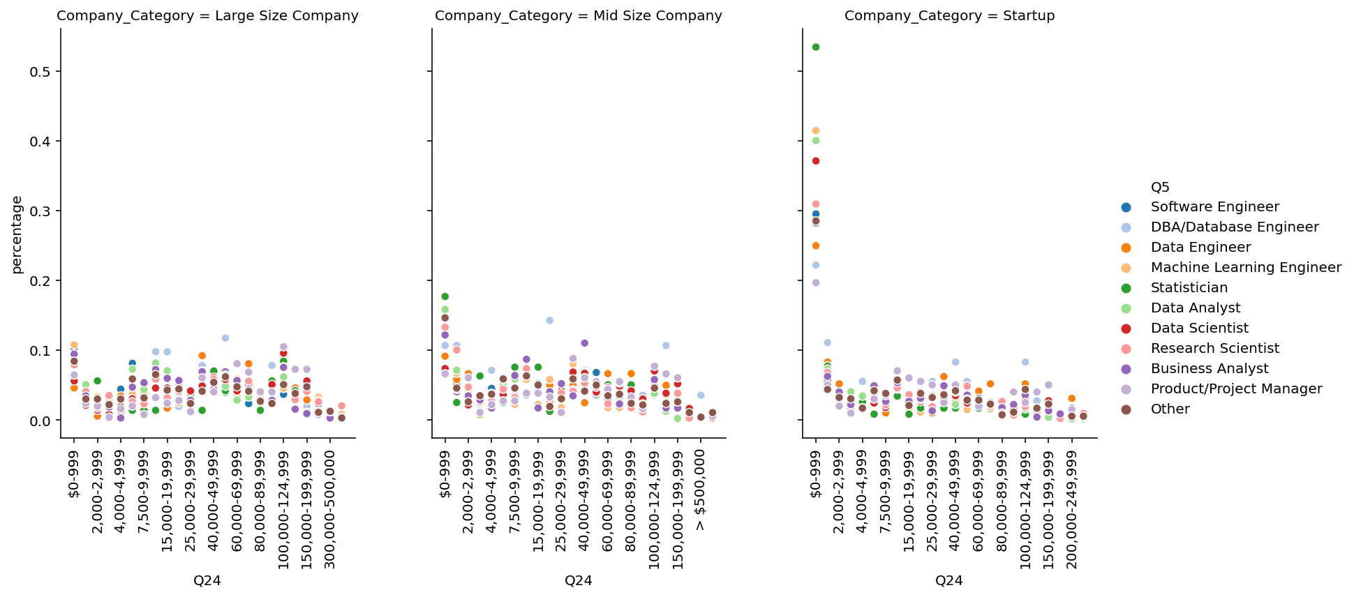
🚀Highlights:
- ~55% staticians of Startup has salary b/w 0-999.
- ~40% Data scientist, Analyst and machine learning developer of Startups has salary b/w 0-999.
- Overall Startups give less money to staticians, Data scientist, Analyst and machine learning developers compare to Large & Mid Size company
Now Let’s see how salary varies with the gender categories.
code
```python data_sub = data[data['Q2'].isin(['Man','Woman'])] df = data_sub[['Company_Category','Q2', 'Q24_new']].groupby(['Company_Category','Q2']).describe() df = df['Q24_new'] (df.style .background_gradient(subset=['mean'])) ```
| count | mean | std | min | 25% | 50% | 75% | max | ||
|---|---|---|---|---|---|---|---|---|---|
| Company_Category | Q2 | ||||||||
| Large Size Company | Man | 3493.000 | 67140.745 | 97001.144 | 999.000 | 14999.000 | 46910.000 | 89999.000 | 1000000.000 |
| Woman | 608.000 | 51888.600 | 80491.320 | 999.000 | 7499.000 | 29999.000 | 69999.000 | 1000000.000 | |
| Mid Size Company | Man | 2440.000 | 51975.483 | 82024.324 | 999.000 | 7499.000 | 29999.000 | 69999.000 | 1000000.000 |
| Woman | 532.000 | 41772.118 | 80058.746 | 999.000 | 1999.000 | 14999.000 | 49999.000 | 1000000.000 | |
| Startup | Man | 3439.000 | 37113.458 | 83085.053 | 999.000 | 999.000 | 9999.000 | 46910.000 | 1000000.000 |
| Woman | 706.000 | 23793.449 | 51965.554 | 999.000 | 999.000 | 1999.000 | 39999.000 | 1000000.000 |
code
```python data_sub = data[data['Q2'].isin(['Man','Woman'])] df = pd.crosstab([data_sub['Q24'], data_sub['Company_Category'], data_sub['Q2']], []).reset_index() df = df.rename(columns={'__dummy__': 'size'}) df1 = pd.crosstab([data_sub['Company_Category'], data_sub['Q2']], []).reset_index() df1 = df1.rename(columns={'__dummy__': 'total_size'}) df = df.merge(df1, how='inner', on=['Company_Category', 'Q2']) df['percentage'] = df['size']/df['total_size'] palette = sns.color_palette("Paired", len(data_sub['Q2'].unique())) lp = sns.relplot( data=df, x="Q24", y="percentage", hue="Q2", col="Company_Category", kind="line", height=5, aspect=.75, palette=palette, facet_kws=dict(sharex=False), ) lp.set_xticklabels(fontsize=10, rotation=90, step=2) ```
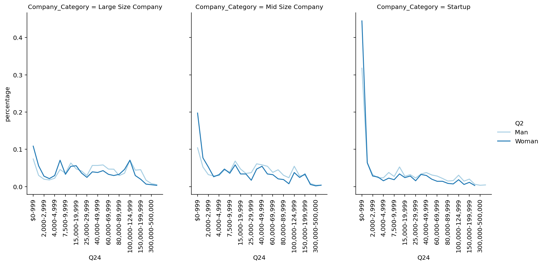
🚀Highlights:
- The average salary of a Man is greater than average salary of woman.
- On Average Man earns 22% more than Woman in Large Size Company where as in Startups difference is 35%
Now Let’s see how salary varies with the highest education taken by respondent.
code
```python df = data[['Company_Category','Q4', 'Q24_new']].groupby(['Company_Category','Q4']).describe() df = df['Q24_new'] (df.style .background_gradient(subset=['mean'])) ```
| count | mean | std | min | 25% | 50% | 75% | max | ||
|---|---|---|---|---|---|---|---|---|---|
| Company_Category | Q4 | ||||||||
| Large Size Company | No formal education past high school | 27.000 | 41655.778 | 31099.823 | 999.000 | 19999.000 | 29999.000 | 64999.000 | 99999.000 |
| Some college/university study without earning a bachelor’s degree | 82.000 | 64647.110 | 72915.418 | 999.000 | 14999.000 | 46910.000 | 97499.000 | 500000.000 | |
| Bachelor’s degree | 1164.000 | 47513.050 | 71769.927 | 999.000 | 7499.000 | 24999.000 | 59999.000 | 1000000.000 | |
| Master’s degree | 2024.000 | 67249.131 | 93095.598 | 999.000 | 14999.000 | 46910.000 | 89999.000 | 1000000.000 | |
| Doctoral degree | 651.000 | 95438.639 | 130908.668 | 999.000 | 24999.000 | 59999.000 | 124999.000 | 1000000.000 | |
| Professional degree | 173.000 | 56355.150 | 107037.022 | 999.000 | 7499.000 | 24999.000 | 49999.000 | 1000000.000 | |
| I prefer not to answer | 51.000 | 70274.627 | 194255.147 | 999.000 | 999.000 | 14999.000 | 49999.000 | 1000000.000 | |
| Mid Size Company | No formal education past high school | 29.000 | 34909.724 | 36946.337 | 999.000 | 999.000 | 19999.000 | 49999.000 | 124999.000 |
| Some college/university study without earning a bachelor’s degree | 109.000 | 44324.385 | 64384.962 | 999.000 | 2999.000 | 24999.000 | 59999.000 | 500000.000 | |
| Bachelor’s degree | 762.000 | 35174.307 | 43905.655 | 999.000 | 3999.000 | 14999.000 | 49999.000 | 249999.000 | |
| Master’s degree | 1371.000 | 56075.032 | 92992.454 | 999.000 | 7499.000 | 29999.000 | 69999.000 | 1000000.000 | |
| Doctoral degree | 568.000 | 63939.639 | 99034.190 | 999.000 | 4999.000 | 39999.000 | 79999.000 | 1000000.000 | |
| Professional degree | 142.000 | 38251.655 | 47191.591 | 999.000 | 2999.000 | 14999.000 | 59999.000 | 199999.000 | |
| I prefer not to answer | 42.000 | 22666.976 | 26273.561 | 999.000 | 1999.000 | 12499.000 | 45182.250 | 124999.000 | |
| Startup | No formal education past high school | 57.000 | 27503.088 | 44475.788 | 999.000 | 999.000 | 3999.000 | 39999.000 | 199999.000 |
| Some college/university study without earning a bachelor’s degree | 227.000 | 28691.454 | 52773.586 | 999.000 | 999.000 | 2999.000 | 46910.000 | 500000.000 | |
| Bachelor’s degree | 1334.000 | 31005.221 | 92367.311 | 999.000 | 999.000 | 2999.000 | 39999.000 | 1000000.000 | |
| Master’s degree | 1743.000 | 34155.404 | 55711.309 | 999.000 | 999.000 | 9999.000 | 46910.000 | 1000000.000 | |
| Doctoral degree | 573.000 | 53573.141 | 115999.994 | 999.000 | 1999.000 | 19999.000 | 59999.000 | 1000000.000 | |
| Professional degree | 185.000 | 30825.957 | 44857.348 | 999.000 | 999.000 | 9999.000 | 46910.000 | 249999.000 | |
| I prefer not to answer | 89.000 | 26749.056 | 63057.663 | 999.000 | 999.000 | 2999.000 | 29999.000 | 500000.000 |
code
```python df = pd.crosstab([data['Q24'], data['Company_Category'], data['Q4']], []).reset_index() df = df.rename(columns={'__dummy__': 'size'}) df1 = pd.crosstab([data['Company_Category'], data['Q4']], []).reset_index() df1 = df1.rename(columns={'__dummy__': 'total_size'}) df = df.merge(df1, how='inner', on=['Company_Category', 'Q4']) df['percentage'] = df['size']/df['total_size'] palette = sns.color_palette("Paired", len(data['Q4'].unique())) lp = sns.relplot( data=df, x="Q24", y="percentage", hue="Q4", col="Company_Category", kind="scatter", height=5, aspect=.75, palette=palette, facet_kws=dict(sharex=False), ) lp.set_xticklabels(fontsize=10, rotation=90, step=2) ```
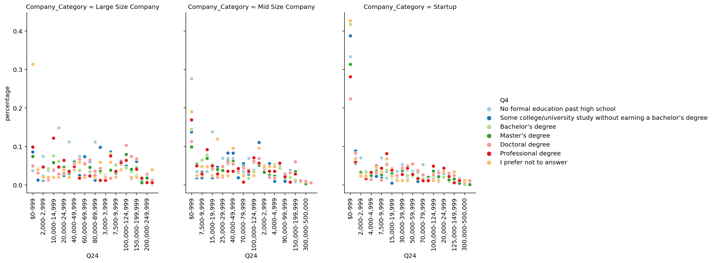
🚀Highlights:
- The average salary of a Doctoral degree is greater.
- There is very small difference in avg Salary of masters and bachelors in Startups, where as large difference in Large and Mid Size Company.
- Avg salary for Professional degree holder in Startups is less than bachelors where as it is more in Large and Mid Size Company.
code
```python df = data[['Company_Category','Q6', 'Q24_new']].groupby(['Company_Category','Q6']).describe() df = df['Q24_new'] (df.style .background_gradient(subset=['mean'])) ```
| count | mean | std | min | 25% | 50% | 75% | max | ||
|---|---|---|---|---|---|---|---|---|---|
| Company_Category | Q6 | ||||||||
| Large Size Company | I have never written code | 222.000 | 45005.248 | 98834.930 | 999.000 | 7499.000 | 24999.000 | 46910.000 | 1000000.000 |
| < 1 years | 384.000 | 37846.539 | 56622.404 | 999.000 | 3999.000 | 14999.000 | 49999.000 | 500000.000 | |
| 1-2 years | 604.000 | 37158.487 | 45042.416 | 999.000 | 4999.000 | 14999.000 | 49999.000 | 249999.000 | |
| 3-5 years | 968.000 | 50016.803 | 79062.026 | 999.000 | 7499.000 | 29999.000 | 69999.000 | 1000000.000 | |
| 5-10 years | 854.000 | 71460.430 | 94127.307 | 999.000 | 19999.000 | 49999.000 | 99999.000 | 1000000.000 | |
| 10-20 years | 660.000 | 96566.029 | 129544.549 | 999.000 | 29999.000 | 69999.000 | 124999.000 | 1000000.000 | |
| 20+ years | 480.000 | 110754.558 | 128806.812 | 999.000 | 39999.000 | 79999.000 | 149999.000 | 1000000.000 | |
| Mid Size Company | I have never written code | 162.000 | 37011.617 | 92715.013 | 999.000 | 1999.000 | 14999.000 | 46910.000 | 1000000.000 |
| < 1 years | 373.000 | 31155.094 | 83376.832 | 999.000 | 1999.000 | 7499.000 | 39999.000 | 1000000.000 | |
| 1-2 years | 487.000 | 29824.735 | 71755.159 | 999.000 | 2999.000 | 9999.000 | 39999.000 | 1000000.000 | |
| 3-5 years | 691.000 | 39623.211 | 45096.085 | 999.000 | 4999.000 | 24999.000 | 59999.000 | 249999.000 | |
| 5-10 years | 557.000 | 55832.594 | 79480.477 | 999.000 | 9999.000 | 39999.000 | 69999.000 | 1000000.000 | |
| 10-20 years | 450.000 | 70391.400 | 80720.265 | 999.000 | 19999.000 | 49999.000 | 89999.000 | 1000000.000 | |
| 20+ years | 303.000 | 98782.152 | 120978.358 | 999.000 | 34999.000 | 79999.000 | 124999.000 | 1000000.000 | |
| Startup | I have never written code | 273.000 | 20271.674 | 32638.859 | 999.000 | 999.000 | 1999.000 | 39999.000 | 199999.000 |
| < 1 years | 649.000 | 19139.891 | 53885.739 | 999.000 | 999.000 | 1999.000 | 24999.000 | 1000000.000 | |
| 1-2 years | 945.000 | 21358.325 | 64684.753 | 999.000 | 999.000 | 1999.000 | 24999.000 | 1000000.000 | |
| 3-5 years | 932.000 | 29021.101 | 81392.880 | 999.000 | 999.000 | 4999.000 | 39999.000 | 1000000.000 | |
| 5-10 years | 576.000 | 40083.932 | 54646.262 | 999.000 | 1999.000 | 19999.000 | 49999.000 | 500000.000 | |
| 10-20 years | 419.000 | 62854.248 | 95953.473 | 999.000 | 6249.000 | 39999.000 | 89999.000 | 1000000.000 | |
| 20+ years | 414.000 | 80057.572 | 127480.974 | 999.000 | 5624.000 | 46910.000 | 99999.000 | 1000000.000 |
code
```python # Q6 df = pd.crosstab([data['Q24'], data['Company_Category'], data['Q6']], []).reset_index() df = df.rename(columns={'__dummy__': 'size'}) df1 = pd.crosstab([data['Company_Category'], data['Q6']], []).reset_index() df1 = df1.rename(columns={'__dummy__': 'total_size'}) df = df.merge(df1, how='inner', on=['Company_Category', 'Q6']) df['percentage'] = df['size']/df['total_size'] palette = sns.color_palette("Paired", len(data['Q6'].unique())) lp = sns.relplot( data=df, x="Q24", y="percentage", hue="Q6", col="Company_Category", kind="scatter", height=5, aspect=.75, palette=palette, facet_kws=dict(sharex=False), ) lp.set_xticklabels(fontsize=10, rotation=90, step=2) ```
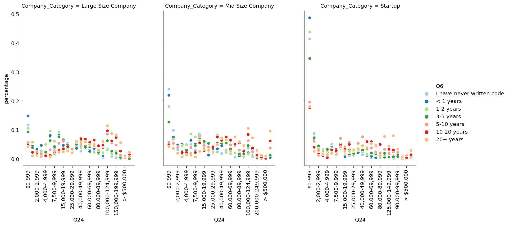
🚀Highlights:
- In All, avg Salary increses with the year of coding experience.
- Avg salary in Startup is less than Mid or Large Size company.
code
```python df = data[['Company_Category','Q15', 'Q24_new']].groupby(['Company_Category','Q15']).describe() df = df['Q24_new'] (df.style .background_gradient(subset=['mean'])) ```
| count | mean | std | min | 25% | 50% | 75% | max | ||
|---|---|---|---|---|---|---|---|---|---|
| Company_Category | Q15 | ||||||||
| Large Size Company | I do not use machine learning methods | 427.000 | 59222.862 | 99546.378 | 999.000 | 7499.000 | 39999.000 | 79999.000 | 1000000.000 |
| Under 1 year | 1004.000 | 43221.308 | 64925.946 | 999.000 | 6874.000 | 19999.000 | 59999.000 | 1000000.000 | |
| 1-2 years | 802.000 | 49030.254 | 57838.133 | 999.000 | 7499.000 | 29999.000 | 69999.000 | 500000.000 | |
| 2-3 years | 502.000 | 65434.530 | 96476.630 | 999.000 | 14999.000 | 46910.000 | 79999.000 | 1000000.000 | |
| 3-4 years | 346.000 | 73905.309 | 112471.381 | 999.000 | 19999.000 | 48454.500 | 89999.000 | 1000000.000 | |
| 4-5 years | 307.000 | 88104.368 | 81829.149 | 999.000 | 29999.000 | 69999.000 | 124999.000 | 500000.000 | |
| 5-10 years | 376.000 | 120033.197 | 143621.043 | 999.000 | 49999.000 | 79999.000 | 149999.000 | 1000000.000 | |
| 10-20 years | 114.000 | 120106.342 | 126344.556 | 999.000 | 49999.000 | 89999.000 | 149999.000 | 1000000.000 | |
| 20 or more years | 72.000 | 153047.222 | 207354.624 | 999.000 | 46910.000 | 89999.000 | 199999.000 | 1000000.000 | |
| Mid Size Company | I do not use machine learning methods | 337.000 | 39642.252 | 66896.277 | 999.000 | 3999.000 | 19999.000 | 49999.000 | 1000000.000 |
| Under 1 year | 804.000 | 35483.867 | 65699.467 | 999.000 | 2999.000 | 14999.000 | 49999.000 | 1000000.000 | |
| 1-2 years | 596.000 | 35959.883 | 43153.827 | 999.000 | 3999.000 | 19999.000 | 49999.000 | 249999.000 | |
| 2-3 years | 373.000 | 57896.954 | 103845.938 | 999.000 | 7499.000 | 39999.000 | 69999.000 | 1000000.000 | |
| 3-4 years | 228.000 | 59134.039 | 61185.089 | 999.000 | 14999.000 | 46910.000 | 79999.000 | 500000.000 | |
| 4-5 years | 210.000 | 70306.410 | 66302.248 | 999.000 | 19999.000 | 54999.000 | 89999.000 | 500000.000 | |
| 5-10 years | 206.000 | 103465.748 | 149086.275 | 999.000 | 26249.000 | 69999.000 | 124999.000 | 1000000.000 | |
| 10-20 years | 66.000 | 95655.409 | 82203.755 | 999.000 | 29999.000 | 89999.000 | 124999.000 | 500000.000 | |
| 20 or more years | 41.000 | 132702.000 | 96074.938 | 999.000 | 49999.000 | 124999.000 | 199999.000 | 500000.000 | |
| Startup | I do not use machine learning methods | 428.000 | 28860.953 | 48139.774 | 999.000 | 999.000 | 9999.000 | 46910.000 | 500000.000 |
| Under 1 year | 1425.000 | 24700.697 | 77560.292 | 999.000 | 999.000 | 1999.000 | 29999.000 | 1000000.000 | |
| 1-2 years | 933.000 | 25164.996 | 51420.469 | 999.000 | 999.000 | 3999.000 | 39999.000 | 1000000.000 | |
| 2-3 years | 431.000 | 40433.441 | 83894.328 | 999.000 | 1999.000 | 14999.000 | 49999.000 | 1000000.000 | |
| 3-4 years | 232.000 | 56312.991 | 105434.274 | 999.000 | 9374.000 | 29999.000 | 69999.000 | 1000000.000 | |
| 4-5 years | 192.000 | 59477.708 | 67260.104 | 999.000 | 7499.000 | 39999.000 | 89999.000 | 500000.000 | |
| 5-10 years | 184.000 | 82851.424 | 105673.430 | 999.000 | 19999.000 | 54999.000 | 106249.000 | 1000000.000 | |
| 10-20 years | 54.000 | 122049.667 | 158252.020 | 999.000 | 46910.000 | 79999.000 | 124999.000 | 1000000.000 | |
| 20 or more years | 56.000 | 132942.304 | 196411.495 | 999.000 | 18749.000 | 69999.000 | 199999.000 | 1000000.000 |
code
```python # Q15 df = pd.crosstab([data['Q24'], data['Company_Category'], data['Q15']], []).reset_index() df = df.rename(columns={'__dummy__': 'size'}) df1 = pd.crosstab([data['Company_Category'], data['Q15']], []).reset_index() df1 = df1.rename(columns={'__dummy__': 'total_size'}) df = df.merge(df1, how='inner', on=['Company_Category', 'Q15']) df['percentage'] = df['size']/df['total_size'] palette = sns.color_palette("Paired", len(df['Q15'].unique())) lp = sns.relplot( data=df, x="Q24", y="percentage", hue="Q15", col="Company_Category", kind="scatter", height=5, aspect=.75, palette=palette, facet_kws=dict(sharex=False), ) lp.set_xticklabels(fontsize=10, rotation=90, step=2) ```
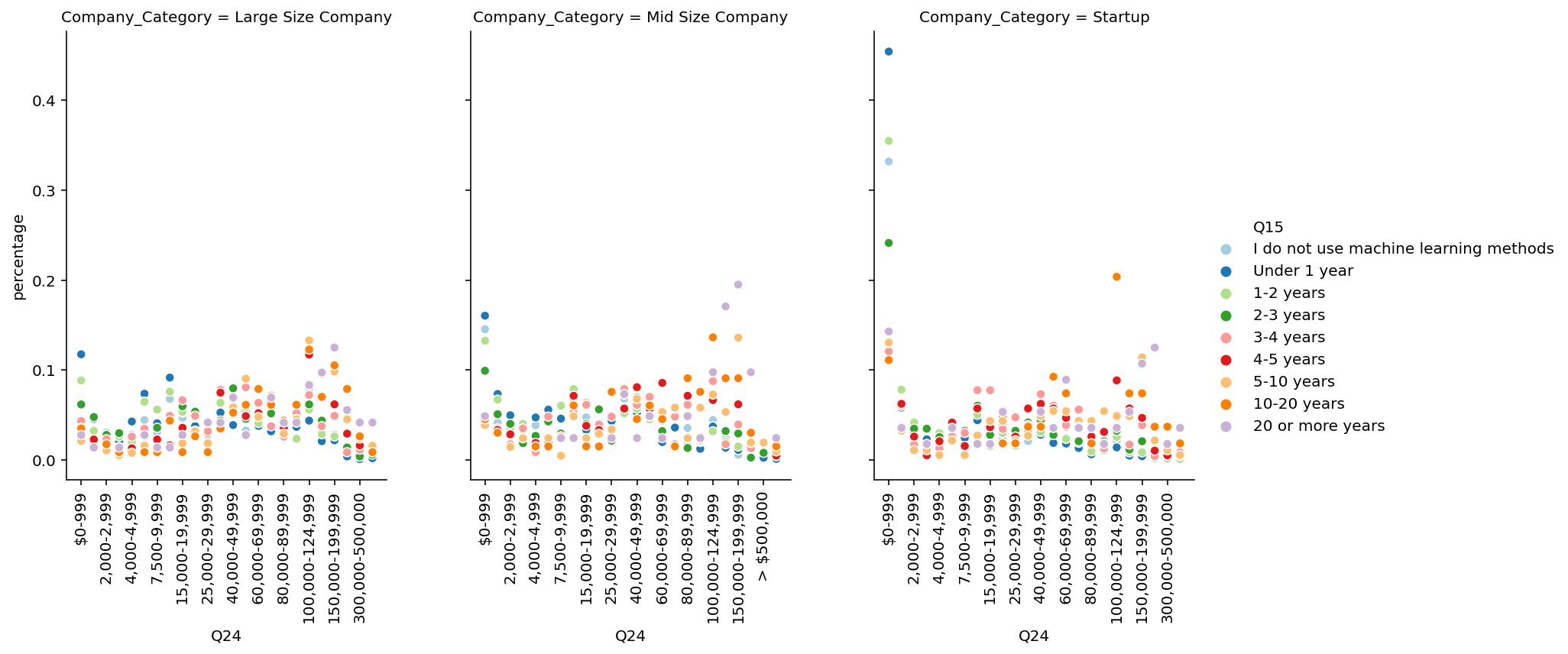
🚀Highlights:
- In All, avg Salary increses with the year of machine learning experience.
- In All, avg Salary of machine learning experience is higher than coding experience.
Summary
| Aspect | Large/Mid Size Company | Startup |
|---|---|---|
| Age | 5 out of 10 has age under 25-35 year and After 55 year, people don’t want to do job in Large or Mid-Size company. | 3 out of 10 has age under 18-24 years. After 55 year, people don’t want to do job for Start-ups. |
| Location | ~40% are from India & USA. | ~30% are from India & USA |
| Education | Has more Mater’s & PhD’s | Has more Bachelors. |
| Job Role | Has more Business Analysts. | Has more Machine learning engineer and Research Scientist. |
| Coding Experience | ~40% of 3-10 year of coding experience. | ~60 of 5 years of coding experience. |
| Machine learning Experience | ~30% of 0-1 year of machine learning experience. | ~40% of 0-1 year of machine learning experience. |
| Programming Language & Packages | SQL & R are more used in Large Size Company. Scikit-Learn, Xgboost, LightGBM, Caret, Catboost are more use in Large Size company. | DL framework i.e. TensorFlow, Keras, Pytorch are more use in Startups. |
| Incorporated Machine Learning | ~25% of them have well established ML methods and models in production for more than 2 years. | ~30% of them are exploring ML methods and may one day put a model into production |
| Opportunities | ~40% of them are building prototypes to explore applying machine learning to new areas. | ~30% of them are building prototypes to explore applying machine learning to new areas. |
| Salary by Job Role | Research Scientist & Data Scientist getting more salary compare to other profiles, avg. salary is $75000-80000. Order is like this: Research Scientist(77741) > Data Scientist(77737) > Machine Learning Engineer(73560) > Statistician(71181) > Data Engineer(63187) > Data Analyst (44106) | Research Scientist & Data Scientist getting more salary compare to other profiles, avg. salary is $40000-45000. \n Order is like this: Data Scientist(41170) > Research Scientist(41550) > Data Engineer(39629) > Machine Learning Engineer(24921) > Statistician(23247) > Data Analyst(22645) |
| Salary by Gender | Man is greater than average salary of woman. Difference in Man vs Woman salary is about 22%. | Man is greater than average salary of woman. Difference in Man vs Woman salary is about 35%. |
| Salary by Education | Avg. Salary of Doctoral degree is greater, whereas large difference in avg. salary of master and bachelors. | Avg. Salary of Doctoral degree is greater, Whereas very small difference in avg. salary of master and bachelors. |
| Salary by ML Experience | Avg. Salary increases with ml experience. | Avg. Salary increases with ml experience. |
References
- moDel Agnostic Language for Exploration and eXplanation: https://github.com/ModelOriented/DALEX
- Line plots on multiple facets: https://seaborn.pydata.org/examples/faceted_lineplot.html
- Color: https://matplotlib.org/3.1.0/tutorials/colors/colormaps.html
- Annotations: https://matplotlib.org/3.3.3/tutorials/text/annotations.html
- Combining two subplots using subplots and GridSpec: https://matplotlib.org/3.1.1/gallery/subplots_axes_and_figures/gridspec_and_subplots.htm
Comments