The Illustrated Network Analysis

knitr::opts_chunk$set(echo = TRUE,message=FALSE,warning=FALSE)

#load packages and csv file
library(ggplot2)
library(dplyr)
library(gridExtra)
library(RColorBrewer)
library(ggthemes)
library(gridExtra)
library(qgraph)
library(igraph)
library(bootnet) 
library(dplyr)
library(NetworkComparisonTest)
library(mgm)

Introduction

In 2013, students of the Statistics class at FSEV UK were asked to invite their friends to participate in this survey.

• The data file (responses.csv) consists of 1010 rows and 150 columns (139 integer and 11 categorical).
• For convenience, the original variable names were shortened in the data file. See the columns.csv file if you want to match the data with the original names.
• The data contain missing values.
• The survey was presented to participants in both electronic and written form.
• The original questionnaire was in Slovak language and was later translated into English.
• All participants were of Slovakian nationality, aged between 15-30.

For this kernel, we use network analysis to analyze the features of HOBBIES & INTERESTS. We use different network analysis techniques and methods to analyze the features.

What is a Network?

• A network is a set of nodes connected by a set of edges
  • Nodes are also called vertices
  • Edges are also called links
  • Networks are also called graphs
• A node represents an entity, this can be anything:
  • People
  • Cities
  • Symptoms
  • Psychological constructs
• An edge represents some connection between two nodes. Again, this can be anything:
  • Friendship / contact
  • Distance
  • Comorbidity
  • Causality
  • Interaction

Types of network

• A network with weighted edges is called a weighted graph
• Otherwise it is called an unweighted graph
• If all edges are directed the network is called a directed graph
• If all edges are not directed the network is called an undirected graph

A directed network with no cycles is called a Directed Acyclic Graph (DAG). A cycle means that you can not start at a node and encounter it again by following directed edges. This includes no self-loops.

DAGs are very useful in that they represent a clear dependency structure between the nodes.

Real World Examples

Causality Analysis

Correlational Structures

In psychometrics, we are often interested in relationships between variables e.g. Correlations, covariances, regression parameters, test statistics, …etc

• Especially correlational structures are important
  • Do items actually measure the same thing?
  • Used to fit factor analysis and structural models

Correlation Visualization Example

• When extended to the amount of variables commonly used in tests
  • Scatterplot and ellipse visualizations become unreadable
  • Heatmaps plots do better, but only show trends Very hard, if not impossible, to see important violations of trends

The Network Approach

• Basic idea:
  • Nodes represent variables
  • Possible to vary in color, shape, size and label to indicate different statistics
• Edges represent relationships
  • Blue edges indicate positive relationships
  • Orange edges indicate negative relationships
  • The wider and more saturated an edge, the stronger the absolute relationship

Network Analysis HOBBIES & INTERESTS of Young People

Loading Young People Survey Data

Data <- read.csv("../input/responses.csv")

Select HOBBIES & INTERESTS features

Data2 <- Data[,32:63] # Select only variables
names(Data2)

Network estimation

Polychoric Correlations

Wikipedia :

In statistics, polychoric correlation is a technique for estimating the correlation between two theorised normally distributed continuous latent variables, from two observed ordinal variables.

This technique is frequently applied when analysing items on self-report instruments such as personality tests and surveys that often use rating scales with a small number of response options (e.g., strongly disagree to strongly agree). The smaller the number of response categories, the more a correlation between latent continuous variables will tend to be attenuated. Lee, Poon & Bentler (1995) have recommended a two-step approach to factor analysis for assessing the factor structure of tests involving ordinally measured items. This aims to reduce the effect of statistical artifacts, such as the number of response scales or skewness of variables leading to items grouping together in factors.

corMat <- cor_auto(Data2) # Correlate data

Unregularized partial correlation network

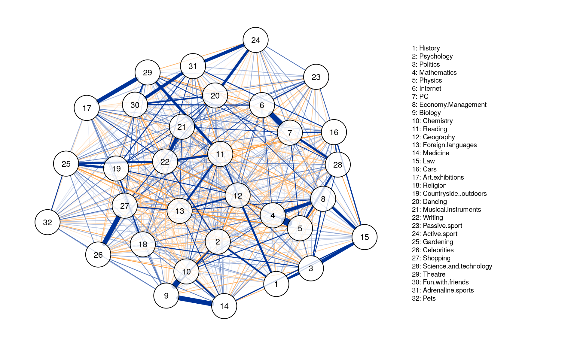
Use the qgraph package in combination with graph = “pcor”.

# Preprocessing of nodes
names<-c("1","2", "3", "4", "5", "6", "7", "8", "9", "10", "11", "12", "13", "14", "15", "16", "17", "18", "19", "20", "21", "22", "23", "24", "25", "26", "27", "28", "29", "30", "31", "32")

Graph_pcor <- qgraph( corMat, graph = "pcor", layout = "spring",
                      tuning = 0.25,sampleSize = nrow(Data2), 
                      legend.cex = 0.35, vsize = 5,esize = 10,
                      posCol = "#003399", negCol = "#FF9933",vTrans = 200, nodeNames = colnames(corMat), labels = names)

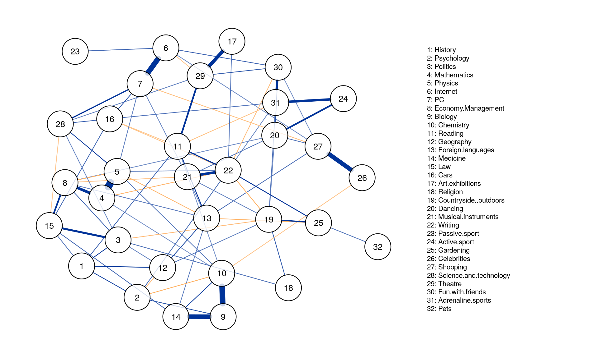
The threshold argument can be used to remove edges that are not significant.

Graph_pcor <- qgraph(corMat, graph = "pcor", layout = "spring", threshold = "bonferroni",
                     sampleSize = nrow(Data2), alpha = 0.05, 
                      legend.cex = 0.35, vsize = 5,esize = 10,
                      posCol = "#003399", negCol = "#FF9933",vTrans = 200, nodeNames = colnames(corMat), labels = names)

#Making igraph object for future processing                      
iGraph_pcor <- as.igraph(Graph_pcor, attributes = TRUE)

Regularized partial correlation network

• Our goal is to obtain:
  • Easily interpretable / parsimoniuous network
  • Stable network that more likely refects our true data generating model

• Solution: Estimate networks with the least absolute shrinkage and selection operator(lasso)

• The lasso shrinks all regression coefficients, and small ones are set to zero (drop out of the model)
  • Interpretability: only relevant edges retained in the network
  • Stability/replicability: avoids obtaining spurious edges only due to chance
  • We also have less parameters to estimate

• Regularization returns a sparse network: few edges are used to explain the covariation structure in the data

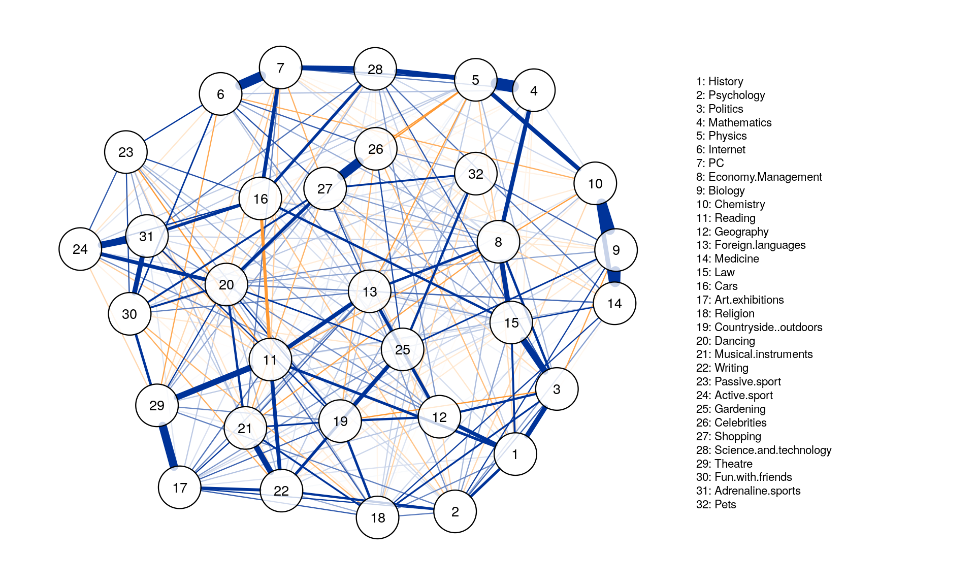
• Estimating a partial correlation network using LASSO regularization and EBIC model selection can be done by setting graph = “glasso”. The tuning argument sets the EBIC hyperparameter. Set between 0 (more connections but also more spurious connections) and 0.5 (more parsimony, but also missing more connections)

Graph_lasso <- qgraph(corMat, graph = "glasso", layout = "spring", tuning = 0.25,
                     sampleSize = nrow(Data2), 
                      legend.cex = 0.35, vsize = 5,esize = 10,
                      posCol = "#003399", negCol = "#FF9933",vTrans = 200, nodeNames = colnames(corMat), labels = names)

---

Observation * The above network gives us some useful information: * The Young People who have interest in `PC`, have also interest in `Internet` and Learning `Science and technology`. * The Young People who have interest in `Mathematics`, have also interest in `Physics`. * The Young People who have interest in `Politics`, have also interest in `Law` and `History`. * The Young People who have interest in `Reading`, have also interest in `Theatre`, `Writing` and `Foreign languages`. * The Young People who have interest in `Cars`, have not interest in `Reading` and vise versa.

---

Centrality Analysis

• Centrality is an important concept when analyzing network graph. The centrality of a node / edge measures how central (or important) is a node or edge in the network.

• We consider an entity important, if he has connections to many other entities. Centrality describes the number of edges that are connected to nodes.

• There many types of scores that determine centrality. One of the famous ones is the pagerank algorithm that was powering Google Search in the beginning.

Computing Centrality Indices

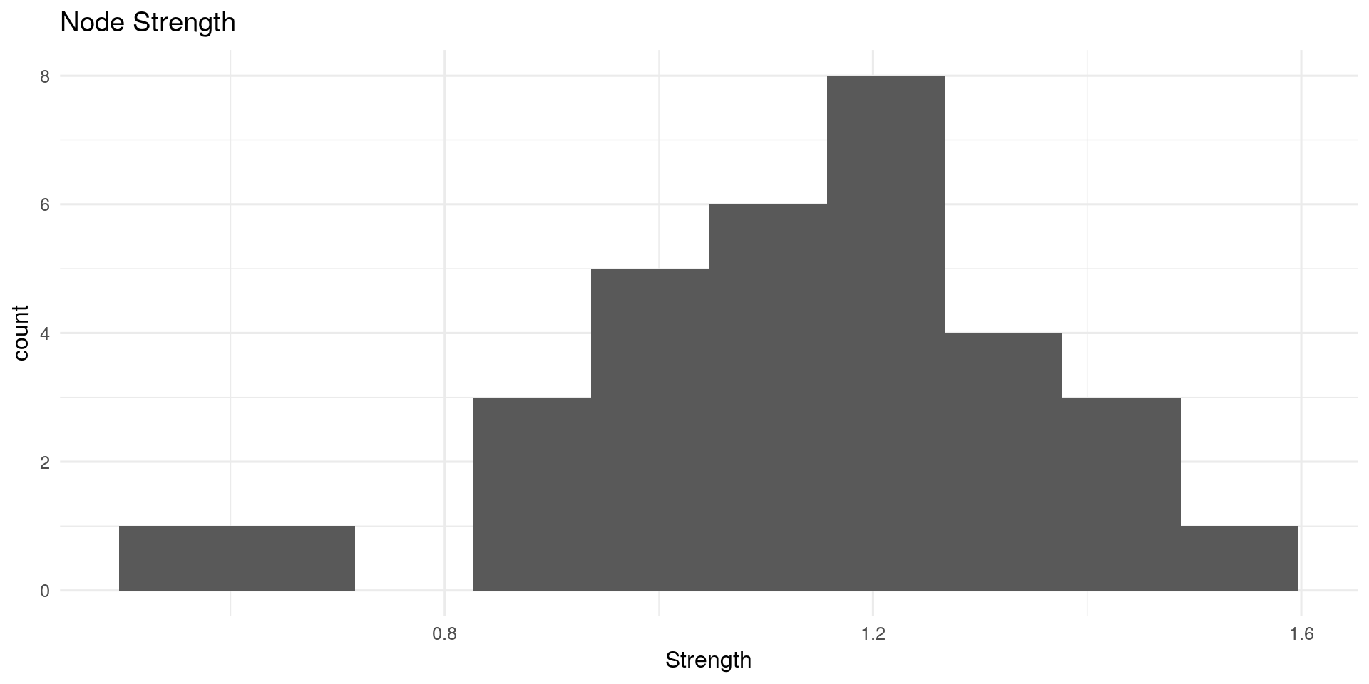
**Node Strength: **

Node strength (also called degree) sums the connected edge weights to a node.

Other possible interpretations: In network of music collaborations, How many people has this person collaborated with?

centRes <- centrality(Graph_lasso)
qplot(centRes$OutDegree, geom = "histogram") + geom_histogram(bins=10) + theme_minimal(12) +
     labs(title="Node Strength") + xlab("Strength")

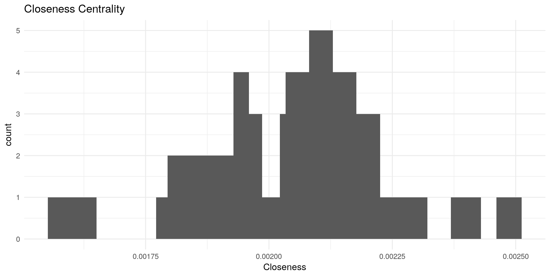
Closeness Centrality:

Closeness centrality measures how many steps is required to access every other nodes from a given nodes. It describes the distance of a node to all other nodes. The more central a node is, the closer it is to all other nodes.

Other possible interpretations: In network of spies, Who is the spy though whom most of the confidential information is likely to flow?

# Closeness:
qplot(centRes$Closeness, geom = "histogram") + geom_histogram(bins=20) + theme_minimal(12) +
     labs(title="Closeness Centrality") + xlab("Closeness")

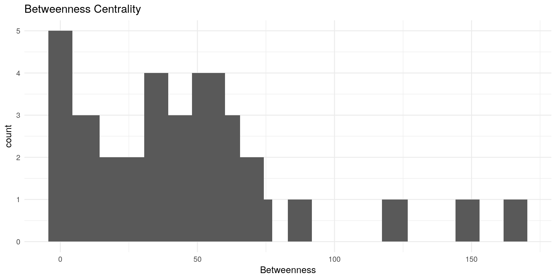
Betweenness Centrality:

The betweenness centrality for each nodes is the number of the shortest paths that pass through the nodes.

Other possible interpretations: In network of sexual relations, How fast will an STD spread from this person to the rest of the network?

# Betweenness:

qplot(centRes$Betweenness, geom = "histogram") + geom_histogram(bins=20) + theme_minimal(12) +
     labs(title="Betweenness Centrality") + xlab("Betweenness")

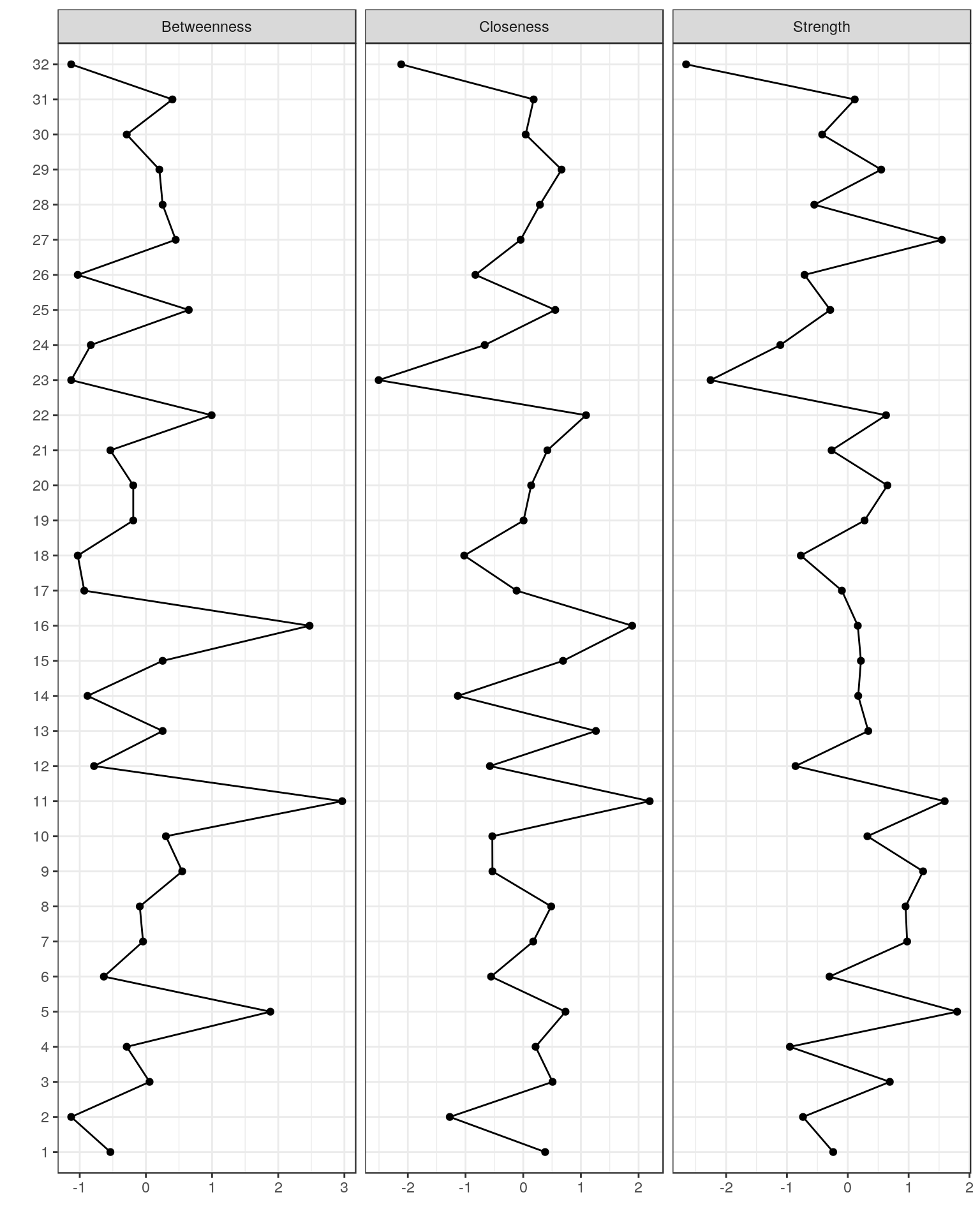
Plotting centrality indices

names(Data2)
centralityPlot(Graph_lasso)

---

Observation * The betweenness centrality for each nodes is the number of the shortest paths that pass through the nodes. `Reading` node has maximum betweenness centrality. * The closeness centrality measures how many steps is required to access every other nodes from a given nodes. `Reading` node has maximum closeness centrality. * The Node strength (also called degree) sums the connected edge weights to a node. `Physics` has maximum strength.

---

centralityPlot(GGM = list(unregularized = Graph_pcor, regularized = Graph_lasso))

---

Observation * The above unregularized vs regularized plot give following information: * In unregularized maximum betweenness node is `Writing` but In regularized maximum betweenness node is `Reading`. * In unregularized maximum closeness node is `Writing` but In regularized maximum closeness node is `Reading`. * In unregularized maximum strength node is `Writing` but In regularized maximum strength node is `Physics`.

---

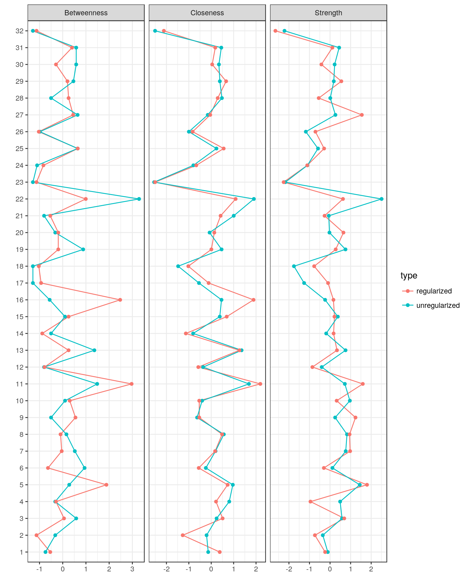
Comparing Graphs

To interpret networks , three values need to be known:

• **Minimum: ** Edges with absolute weights under this value are omitted
• Cut: If specified, splits scaling of width and color
• **Maximum: ** If set, edge width and color scale such that an edge with this value would be the widest and most colorful

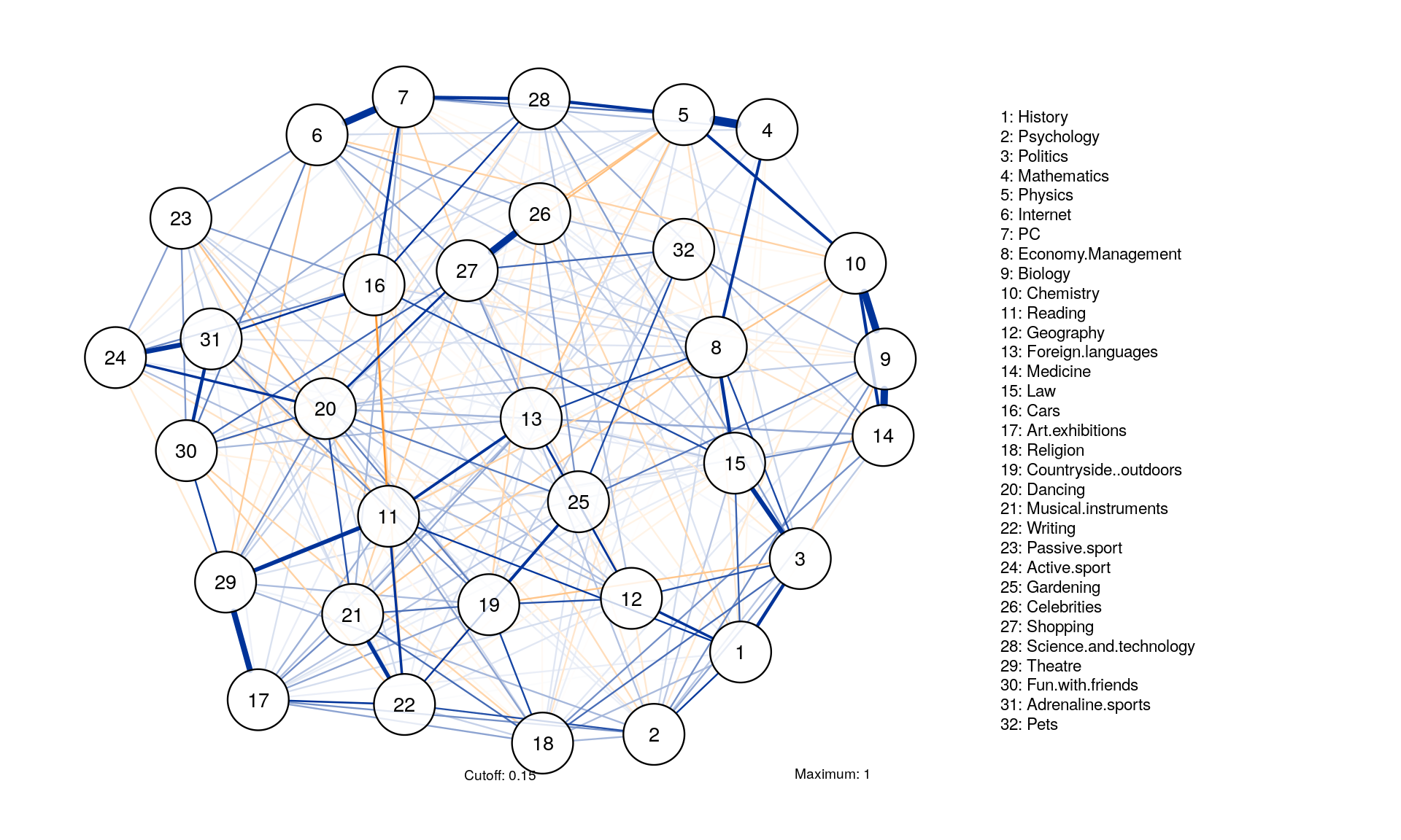
Minimum, maximum and cut

qgraph(corMat, graph = "glasso", layout = "spring", tuning = 0.25,
                     sampleSize = nrow(Data2), minimum = 0,
                      cut = 0.15, maximum = 1, details = TRUE, 
                      legend.cex = 0.35, vsize = 5,esize = 10,
                      posCol = "#003399", negCol = "#FF9933",vTrans = 200, nodeNames = colnames(corMat), labels = names) 

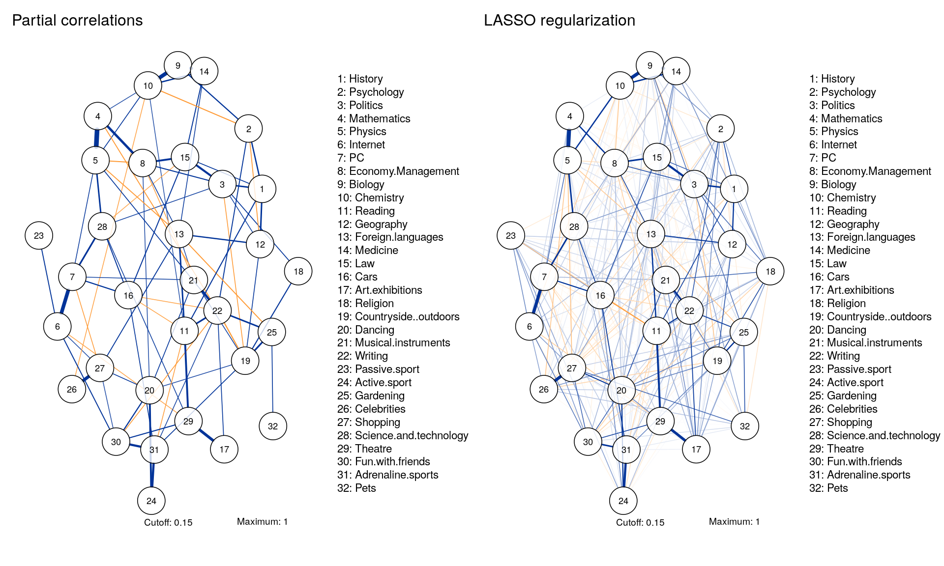
Comparable Layouts

Layout <- averageLayout(Graph_pcor,Graph_lasso)
layout(t(1:2))
qgraph(corMat, graph = "pcor", layout = Layout, threshold = "bonferroni",
                     sampleSize = nrow(Data2), minimum = 0,
                      cut = 0.15, maximum = 1, details = TRUE,
                      title = "Partial correlations", 
                      legend.cex = 0.35, vsize = 5,esize = 10,
                      posCol = "#003399", negCol = "#FF9933",vTrans = 200, nodeNames = colnames(corMat), labels = names)

qgraph(corMat, graph = "glasso", layout = Layout, tuning = 0.25,
                     sampleSize = nrow(Data2), minimum = 0,
                      cut = 0.15, maximum = 1, details = TRUE,
                      title = "LASSO regularization", 
                      legend.cex = 0.35, vsize = 5,esize = 10,
                      posCol = "#003399", negCol = "#FF9933",vTrans = 200, nodeNames = colnames(corMat), labels = names)

Eigenvalue Decomposition

Traditionally, we would want to describe the 32 items above in a latent variable framework, and the question arises: how many latent variables do we need to explain the covariance among the 32 items? A very easy way to do so is to look at the eigenvalues of the components in the data.

plot(eigen(corMat)$values, type="b",ylab ="Eigen Value" )
abline(h=1,col="red", lty = 3)

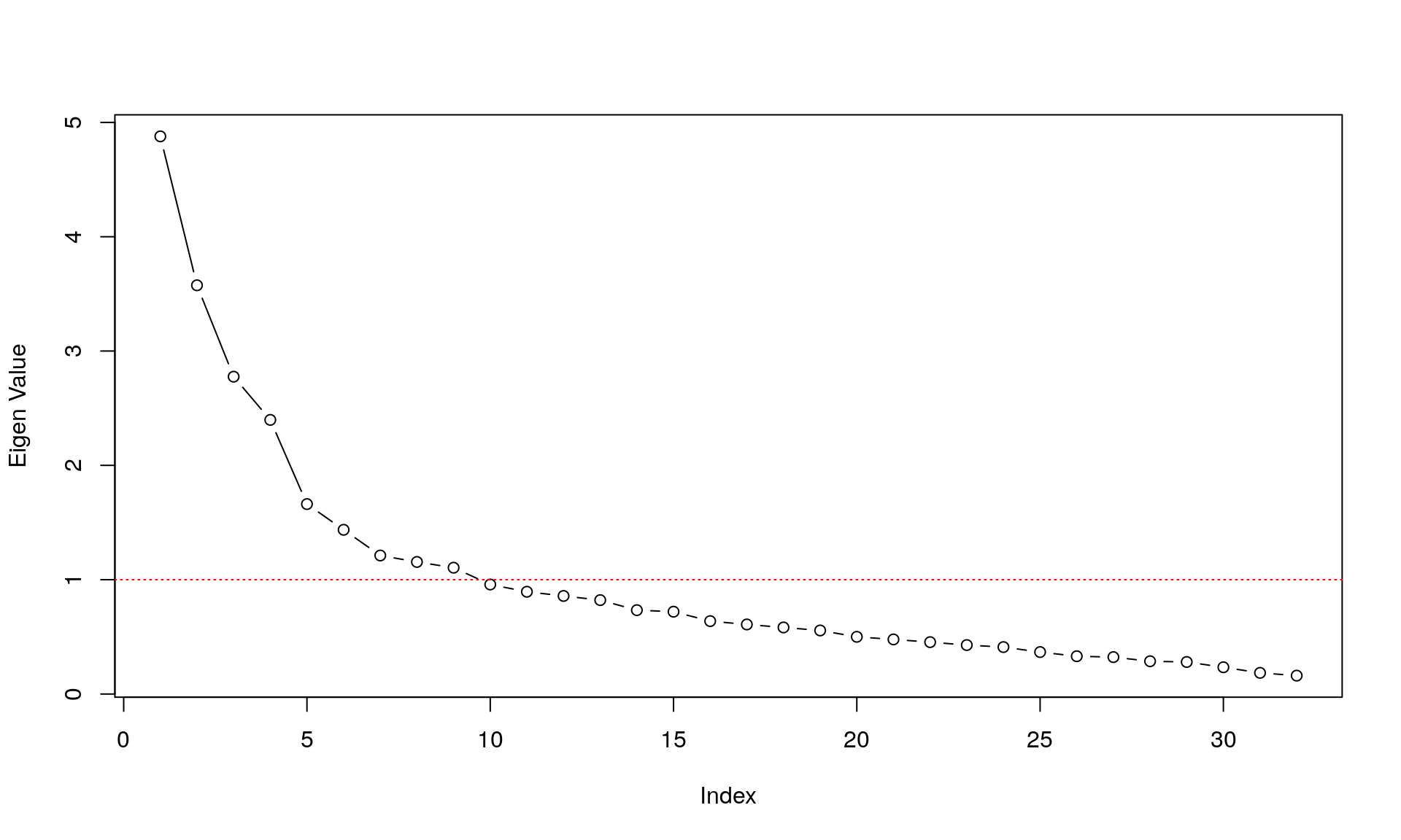
This shows us the value of each eigenvalue of each components on the y-axis; the x-axis shows the different components. A high eigenvalue means that it explains a lot of the covariance among the items. The red line depicts the so-called Kaiser criterion: a simple rule to decide how many components we need to describe the covariance among items sufficiently (every components with an eigenvalue > 1).

Clustering

• Clustering is a common operation in network analysis and it consists of grouping nodes based on the graph topology.

• It’s sometimes referred to as community detection based on its commonality in social network analysis.

• Quick summary of community detection algorithms availabel in igraph

  • cluster_walktrap() Community strucure via short random walks, see http://arxiv.org/abs/physics/0512106
  • cluster_edge_betweenness() aka Girvan-Newman algorithm: Community structure detection based on edge betweenness. Consecutively each edge with the highest betweenness is removed from the graph.
  • cluster_fast_greedy() aka Clauset-Newman-Moore algorithm. Agglomerative algorithm that greedily optimises modularity. Fast, but might get stuck in a local optimum.
  • cluster_spinglass() Finding communities in graphs based on statistical meachanics
  • cluster_leading_eigen() Community structure detecting based on the leading eigenvector of the community matrix – splits into two communities?
  • cluster_infomap() Minimizes the expected description length of a random walker trajectory
  • cluster_label_prop() Fast – Find communities by contagion: propagating labels, updating the labels by majority of neighbors
  • cluster_louvain() Fast, hierarchical. Each vertex is moved to the community with which it achieves the highest contribution to modularity (agglomeration in k-means?)
  • cluster_optimal() Slow, optimal communities based on maximal modularity score.

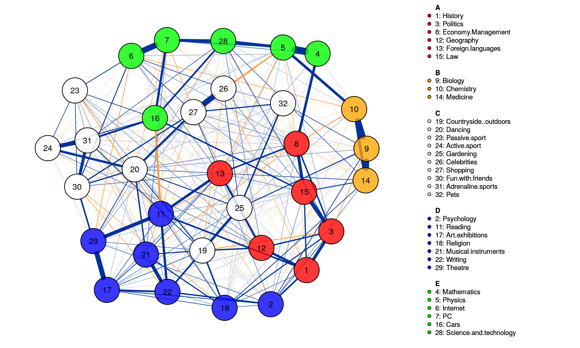
Spinglass Community

This method is the so-called spinglass algorithm that is very well established in network science. For that, we feed the network we estimated above to the igraph R-package. The most relevant part is the last line sgc$membership.

g = as.igraph(Graph_lasso, attributes=TRUE)
sgc <- spinglass.community(g)
sgc$membership

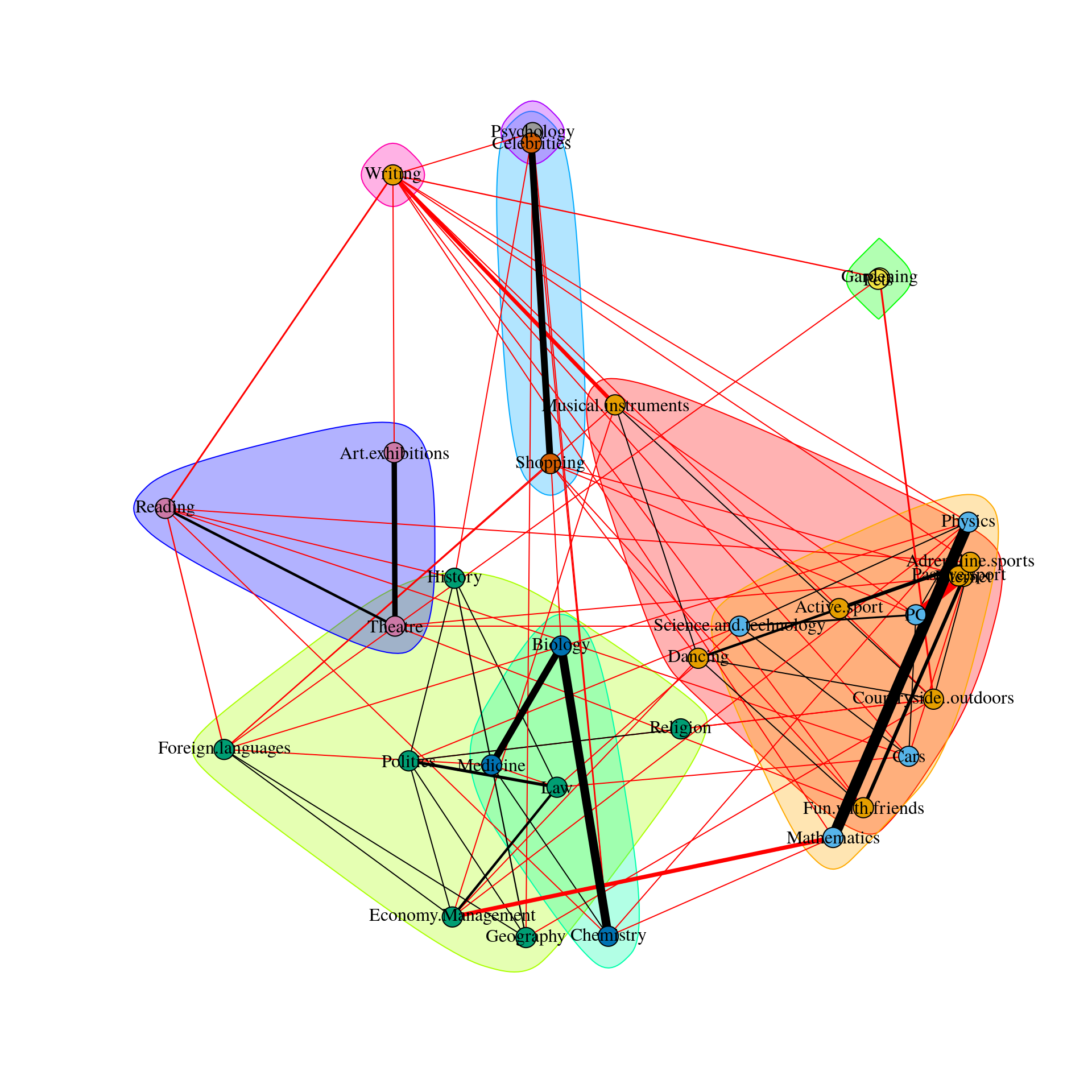
This means the spinglass algorithm detects 5 communities, and this vector represents to which community the 32 nodes belong

We can then easily plot these communities in qgraph by, for instance, coloring the nodes accordingly. Note that iqgraph is a fantastically versatile package that has numerous other possibilites for community detection apart from the spinglass algorithm, such as the walktrap algorithm. (Thanks to Alex Millner for his input regarding igraph; all mistakes here are my mistakes nonetheless, of course).

group.spinglass<- list(c(1,3,8,12,13,15), c(9,10,14), c(19,20,23,24,25,26,27,30,31,32), c(2,11,17,18,21,22,29), c(4,5,6,7,16,28))
Graph_lasso <- qgraph(corMat, graph = "glasso", layout = "spring", tuning = 0.25,
                     sampleSize = nrow(Data2), 
                      legend.cex = 0.35, vsize = 5,esize = 10,
                      posCol = "#003399", negCol = "#FF9933",vTrans = 200,groups=group.spinglass,color=c("red", "orange", "white", "blue", "green"),nodeNames = colnames(corMat), labels = names)

Walktrap Community

• This algorithm finds densely connected subgraphs by performing random walks. The idea is that random walks will tend to stay inside communities instead of jumping to other communities.

• Dense subgraphs of sparse graphs (communities), which appear in most real-world complex networks, play an important role in many contexts. Computing them however is generally expensive. We propose here a measure of similarities between vertices based on random walks which has several important advantages: it captures well the community structure in a network, it can be computed efficiently, and it can be used in an agglomerative algorithm to compute efficiently the community structure of a network. We propose such an algorithm, called Walktrap, which runs in time O(mn^2) and space O(n^2) in the worst case, and in time O(n^2log n) and space O(n^2) in most real-world cases (n and m are respectively the number of vertices and edges in the input graph). Extensive comparison tests show that our algorithm surpasses previously proposed ones concerning the quality of the obtained community structures and that it stands among the best ones concerning the running time.

plot(
    cluster_walktrap(iGraph_pcor), 
    as.undirected(iGraph_pcor), 
    vertex.size = 5,
    vertex.label = colnames(corMat)
  )

Replicability

We all know that all our work should be replicable, especially outputs, but exactly how replicable does something need to be?

#Data preparation

### Obtain two different datasets:
data1 <- slice(Data2, c(1:505))    # n = 505
data2 <- slice(Data2, c(506:1010))   # n = 506

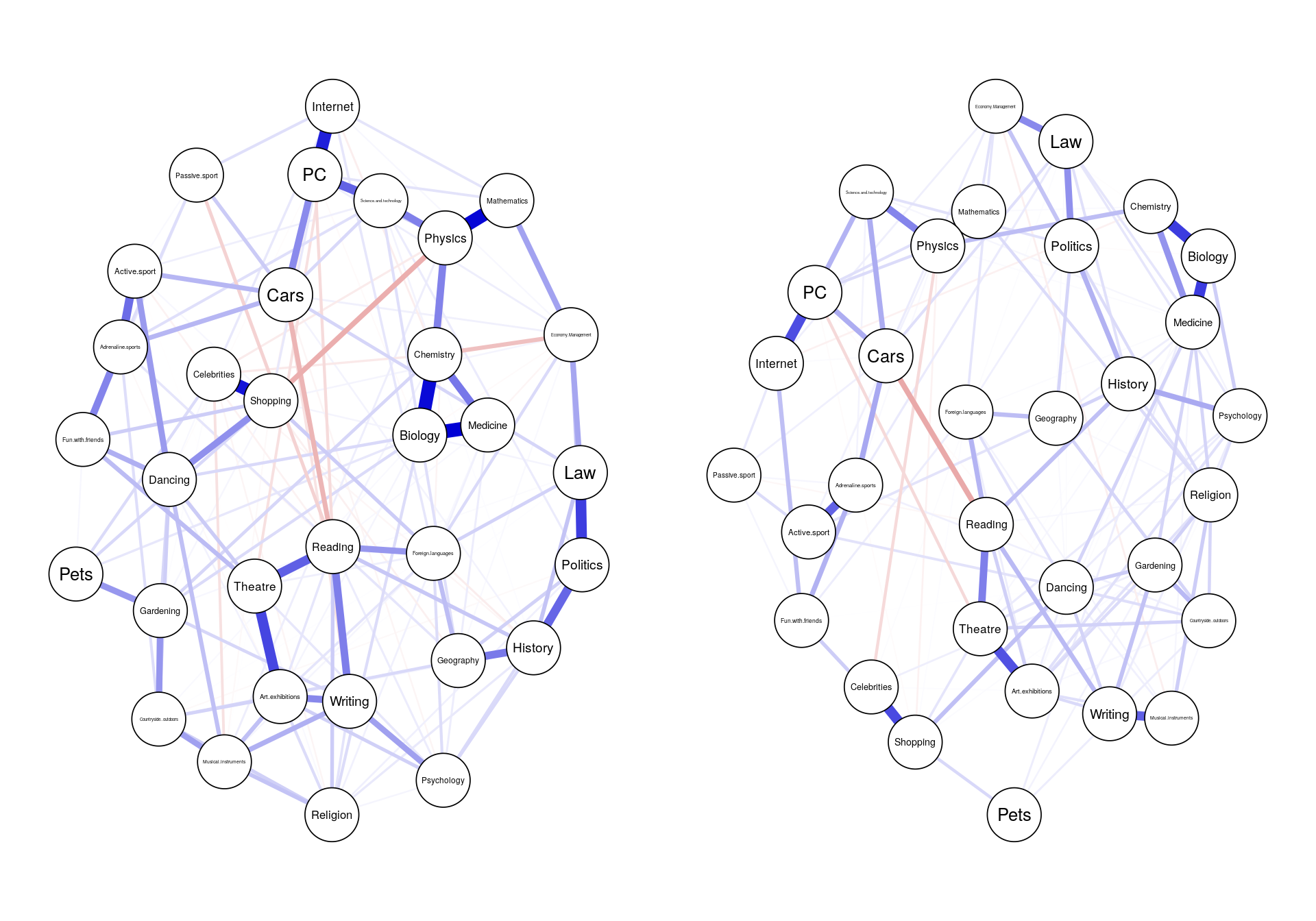
### similarity: visual
network1 <- estimateNetwork(data1, default="EBICglasso")
network2 <- estimateNetwork(data2, default="EBICglasso")

layout(t(1:2))
graph1 <- plot(network1, cut=0)
graph2 <- plot(network2, cut=0)

### similarity: statistical
cor(network1$graph[lower.tri(network1$graph)], network2$graph[lower.tri(network1$graph)], method="spearman")

cor(centrality(network1)$InDegree, centrality(network2)$InDegree)

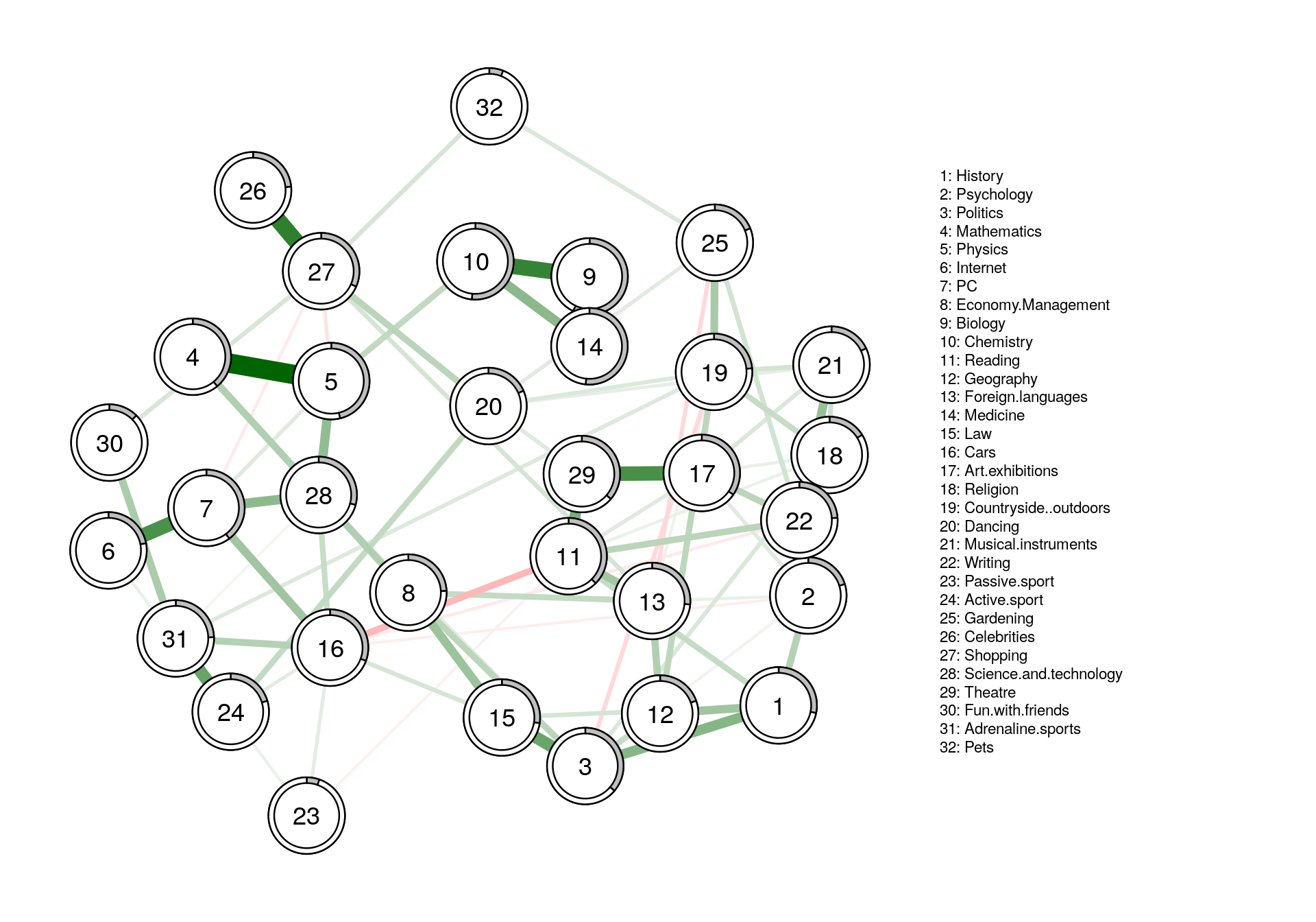
Predictability

• How much variance of a given node can be explained by its neighbors?
• How self-determined is a system?
• While centrality is a relative metric, predictablility is absolute

#Data preparation

for(i in 1:ncol(Data2)){
  Data2[is.na(Data2[,i]), i] <- median(Data2[,i], na.rm = TRUE)
}

corMat2 <- corMat
corMat2[1,2] <- corMat2[2,1] <- corMat[1,2] + 0.0001 # we change the correlation matrix just a tiny little bit
L1 <- averageLayout(corMat, corMat2)

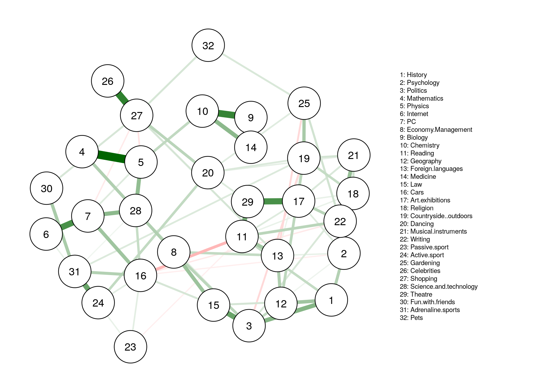
#making model
fit <- mgm(Data2, type=rep('g',32), level=rep(1,32), k=2, lambdaSel = 'EBIC', 
            lambdaGam = 0.25)

#plotting
fit_plot <- qgraph(fit$pairwise$wadj, cut=0, legend.cex = 0.35,
                    layout = L1, edge.color = fit$pairwise$edgecolor, nodeNames = colnames(corMat), labels = names )

#predict
pred_obj <- predict(object = fit, 
                    data = Data2, 
                    errorCon = 'R2')

#error
pred_obj$error

#plotting with error in pie chart
fit_plot2 <- qgraph(fit$pairwise$wadj, cut=0, pie = pred_obj$error[,2],legend.cex = .35,
                    layout = L1, edge.color = fit$pairwise$edgecolor, nodeNames = colnames(corMat), labels = names)

Appendix

Polychoric correlation

Weighted Network

Strength of Nodes

Network Analysis

Graph-based Predictable Feature Analysis

Replicability

Run In Notebook

Kaggle Notebook